Insert PivotChart In Excel: A Complete Guide
Mar 28, 2023
Do you want an effective way to summarize large data sets in Excel?
Learning to insert a PivotChart in Excel can help bring value to how you manage the most complex data sets. With a few simple steps, you can quickly present and analyze large amounts of data, giving yourself insight into trends or patterns that would otherwise stay hidden!
Read on as we cover the following:
-
What Is a PivotChart?
-
How to Create a PivotChart
-
Final Thoughts on How to Insert a PivotChart in Excel
-
Frequently Asked Questions on How to Insert a PivotChart in Excel
What Is a PivotChart?
PivotChart or Excel PivotChart is a graphic or visual representation of the data. PivotCharts give you the complete picture of your summary data source.
PivotChart also lets you analyze data using graphs and layouts. PivotChart is best suited for a company presentation of extensive sales data.
Read Also: Ultimate Excel PivotTables Tutorial: Beginner to Advanced
How to Create a PivotChart
There are two ways to create a PivotChart:
-
Create a PivotChart from a data sheet without a PivotTable
-
Create a PivotChart with an existing PivotTable
Create a PivotChart from a Data Sheet without PivotTables
-
Go to the Insert tab and click PivotChart.

-
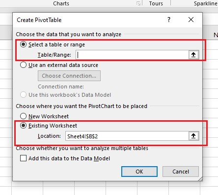
In the Create PivotTable dialog box, click "Select a table or range" instead of "Use an external data source." Choose a cell from the new chart sheet to where you want the PivotChart.
-
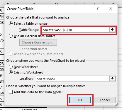
Select the data range from the other data sheet to create a pivot chart and click ok.
-
A blank pivot table will appear. Set up your PivotChart Fields.
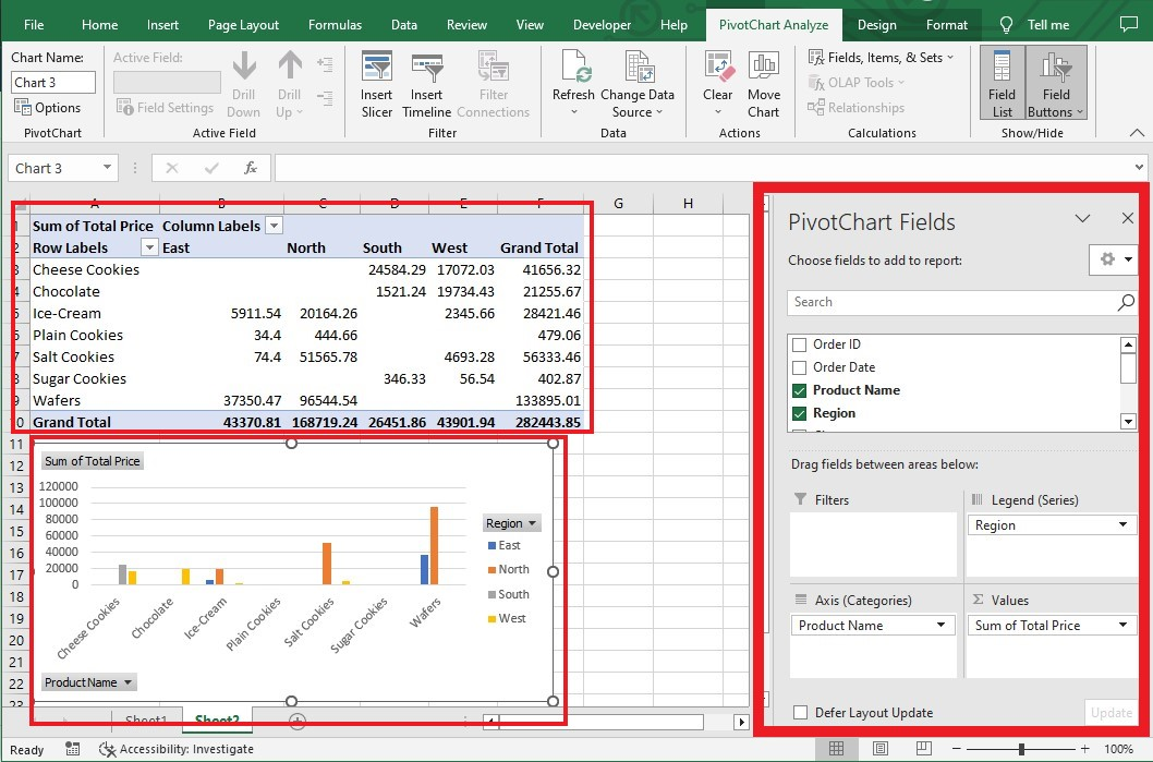
Excel will automatically create a PivotChart once you've finished setting up the PivotChart fields pane.
Create a PivotChart with Existing PivotTables
-
Click any cell in the Pivot Table.
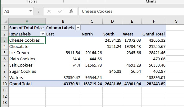
-
Go to the Insert tab, and click PivotChart.

-
You will see many charts in the Insert Chart dialog box. Choose a chart type that fits your Pivot Table's data and click OK.
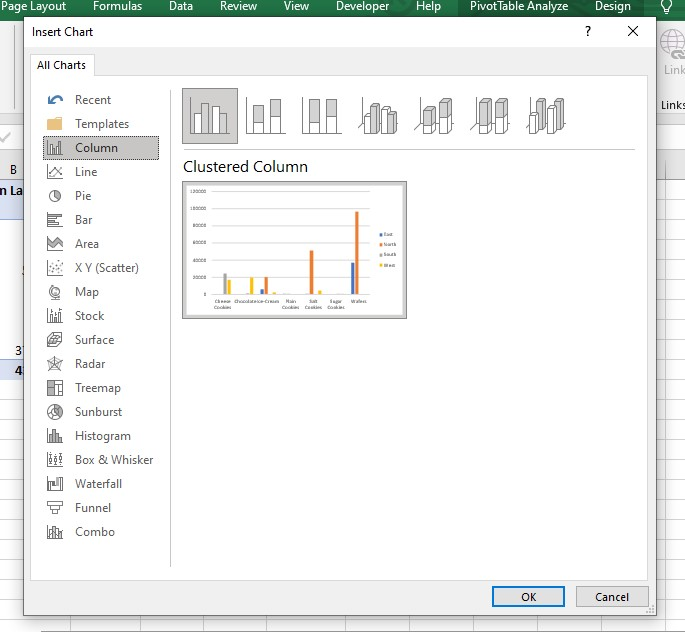
The dialog box will create a PivotChart with the source data from the Pivot Table.
Final Thoughts on How to Insert a PivotChart In Excel
With all that you have learned about inserting a PivotChart in Excel, you are now ready to start visualizing your data in a new way. You can create dynamic visuals to analyze and present information effectively.
For more easy-to-follow Excel guides and the latest Excel Templates, visit Simple Sheets and the Related Articles section of this blog post.
Subscribe to Simple Sheets on YouTube for the most straightforward Excel video tutorials!
Frequently Asked Questions on Insert PivotChart In Excel
How can I add chart elements to my PivotChart?
Click the + button on the right of your PivotChart to add chart elements like axis titles, gridlines, legends, and many more. You can also change the position of your chart elements.
How can I format my PivotChart?
Using the PivotChart tools, you can format your chart sheet. The PivotChart tools provide formatting options for colors, backgrounds, and fonts. You can also add new fields and perform other functions to make your chart look more excellent than before.
How do I add a slicer for my PivotChart?
-
Click your PivotChart.
-
Go to the Analyze tab, and click Insert Slicer.
-
Create the slicers in the Select Fields dialog, and click Ok.
Related Articles:
How to Connect Slicers to Multiple PivotTables
Excel PivotTable Training: Everything You Need to Know
A Reference Isn't Valid Excel Error | How to Fix this Error?
Want to Make Excel Work for You? Try out 5 Amazing Excel Templates & 5 Unique Lessons
We hate SPAM. We will never sell your information, for any reason.


