Everything You Need to Learn on Auditing Formulas in Excel

Are you looking for ways to save time and become more efficient with data management?

Excel formulas are the perfect solution. They allow users to perform complex calculations within seconds.

However, errors can easily creep in when dealing with large amounts of data. So, it's important to audit your formulas regularly.

In this blog post, we'll show you how to audit your Excel formulas properly, ensuring accurate results every time. 

Here's what to expect from this article:

• What Is Formula Auditing?

• Features of Formula Auditing

• Things to Remember when Auditing Formulas in Excel

• Final Thoughts on Auditing Formulas in Excel

• Frequently Asked Questions on Auditing Formulas in Excel

What Is Formula Auditing?

You can conduct formula auditing in Excel to determine the relationship between cells and formulas.

Moreover, the Excel Formula Auditing tools help you identify the following:

• The cells contribute to solving a formula present in the active cell.

• The formulas that based on the active cell.

The output of Formula Auditing is shown graphically by arrow lines, making the entire formula visualization easy.

Besides, it shows the formulas in the active spreadsheet with a single command. So, if your formulas refer to cells shown in a different workbook, you will see that particular source sheet.

Microsoft Excel provides various ways to audit a formula. Moreover, you will find the Formula Auditing group if you click the Excel Formulas tab.

However, many users might need to customize the ribbon to see this option. Here are the different options for auditing a formula:

• Trace Precedents

• Trace Dependents

• Remove Arrows

• Show Formulas

• Error Checking

1. Trace Precedents option

Trace Precedents display tracer arrows from the cells showing the direction of information flow. A blue box fills the cells when this option is active.

However, you can click this button multiple times to catch additional levels.

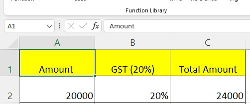
As shown in the above table, we are given a formula in the C2 cell for calculating the GST amount for your Service amount.

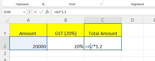
Double-click cell C2, the required cell. You will observe that the precedents cells got bordered with various colors and typed in the same color and cell reference.

You will notice that cell A2 is blue, and the border color also uses the same hue.

Though it is easy, we have a more suitable way to check precedents for the formula cell.

Here are the steps to use the "Trace Precedents" option in your Excel worksheet:

1. Choose a cell.

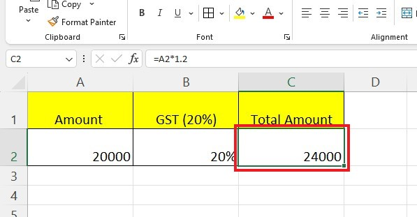
2. Go to the Formulas tab. In the "Formula Auditing" group, click the "Trace Precedents" option.

3. The outcome will be an arrow, as shown below.

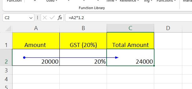
In the above image, the precedent cells appear with blue dots.

2. Trace Dependents option

The Trace Dependents option in Excel helps you determine which formulas use a certain number.

For example, if one number uses in many formulas, select the formula cell and click Trace Dependents. All the cells with that number will be blue, with arrows pointing to all the places.

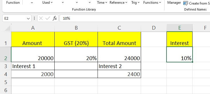
We have calculated the 10% interest for the base and GST amounts, as shown in the example below:

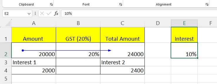
We used a formula to calculate the number in the first and second cells. The formula uses E2 as part of it, which means that E2 depends on A4 and C4. To use Trace Dependents for cell E2, follow these steps:

1. Choose the dependent cell E2.

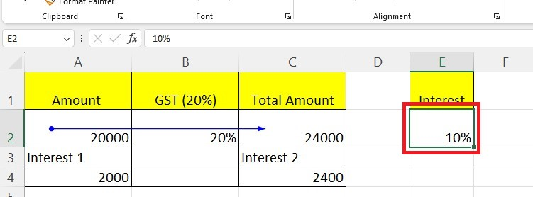
2. Go to the"Formulas" tab. In the "Formula Auditing" group, click the "Trace Dependents" option.

3. In the outcome, you will see two arrows shown from cells E2 to A4 and cells E2 to C4. Meanwhile, A4 and C4 are based on E2.

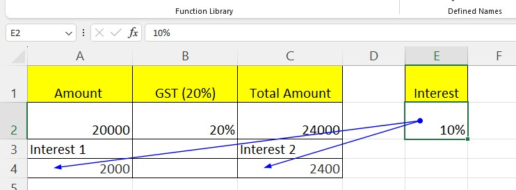
Later, if you want to remove these arrows, you can use the "Remove Arrows" option in the same section.

3. Remove Arrows options

Earlier, we talked about Trace Precedent and Trace Dependent. We used these methods to show arrows in cells which show how information moves.

Excel can do it quickly if you want to remove the arrows later. Here is how you can remove the arrows from cell E2:

1. Go to the "Formulas" tab. In the "Formula Auditing" group, click the "Remove Arrow" option.

2. Every arrow from the active Excel worksheet will fade in the outcome.

4. Showing Formulas option

It is important to ensure everything works properly with Excel and many formulas. A "Show Formula" option will quickly show all the formula cells in your worksheet so you can check them.

The worksheet below contains the GST report and our base amount's 10% interest figure.

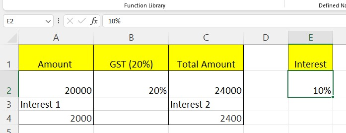
Here we have typed the formula in three of the cells. Following are the ways to show all the cells having formulas in your active Excel worksheet:

1. Go to the "Formulas" tab. In the "Formula Auditing" group, click the "Show Formulas" option.

2. The formulas in the worksheet will appear for you. You can see which cells have a formula and what the formula is. Look at the picture to see all of the formulas.

5. Evaluating a Formula option

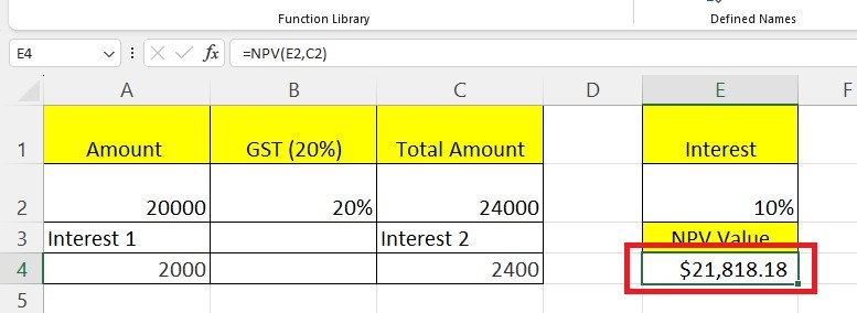
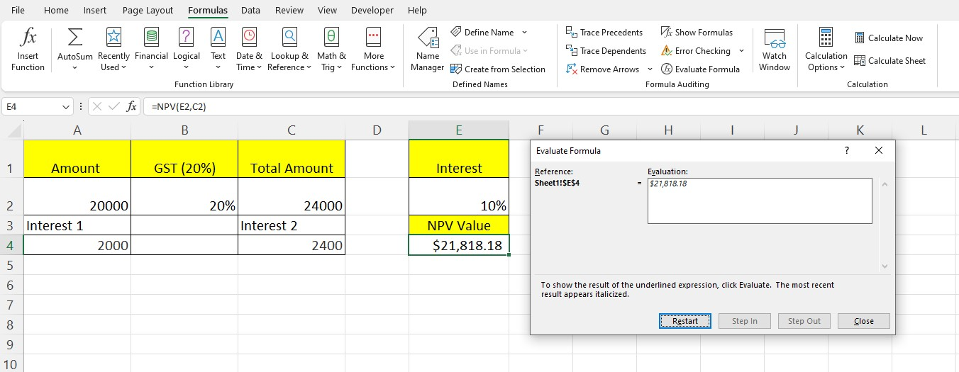
Sometimes, you get sheets with complicated formulas. You can use the Excel "Evaluate Formula" command to see how the formula works. For example, if there is an NPV formula in cell E4, here's what you do:

1. Click on the formula cell E4.

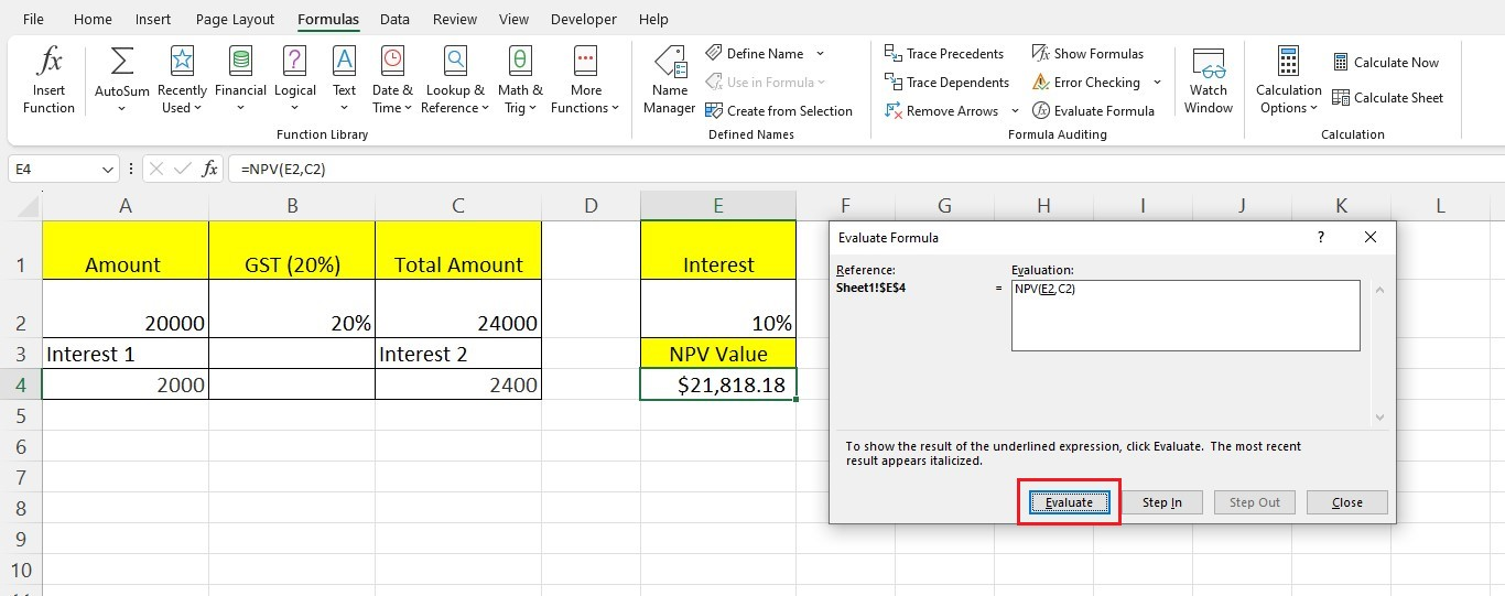
2. Go to the "Formulas" tab. In the "Formula Auditing" group, click the "Evaluate Formula" option.

3. The "Evaluate Formula" dialog box will appear. In the Evaluate Formula dialog box, the formula used in the specified cell appears in the box under evaluation.

4. Click evaluate formula button many times. It will let Excel give you a step-by-step evaluation of the formula. Moreover, it will present the result of the underlined expression.

5. Once you're done, the "Evaluate" button will change to the "Restart" button.

6. Error Checking option

When using formulas and functions, it is easy to make mistakes. So, checking the formula errors is important.

Furthermore, you must check your work carefully after completing all the calculations. Here's an example of checking for errors:

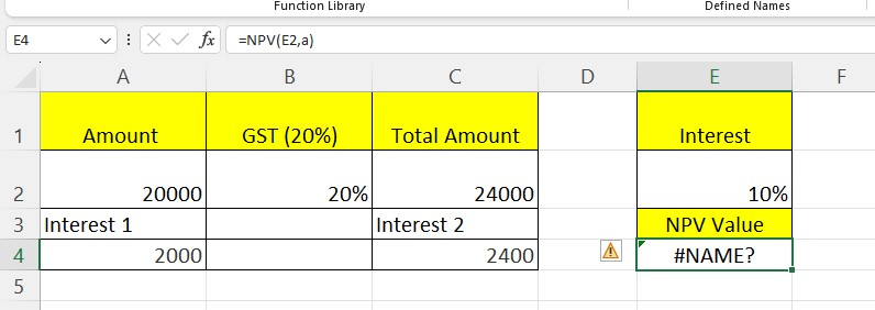
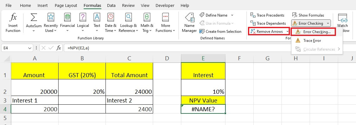
In cell E4, you will see an error called "#NAME?". You can do the "Error Checking" option to determine what is wrong. Here's how it works:

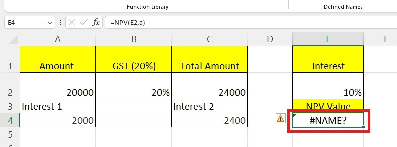
1. Click the cell that has an error message.

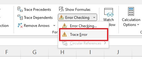
2. Go to the "Formulas" tab. In the "Formula Auditing" group, click the arrow next to the "Error Checking" option.

3. You will see three choices in the list: Error-checking, Trace errors, and Circular References. In this case, the third option is gray, meaning there are no circular references in the Excel workbook.

4. Choose the "Trace Error" option from the drop-down menu.

5. Blue arrows represent the cells required to compute the active cell.

6. Click the "Remove Arrows." Again, click the drop-down arrow next to the "Error Checking" option. From the drop-down options, select the Error Checking option.

7. The Error Checking dialog box will appear.

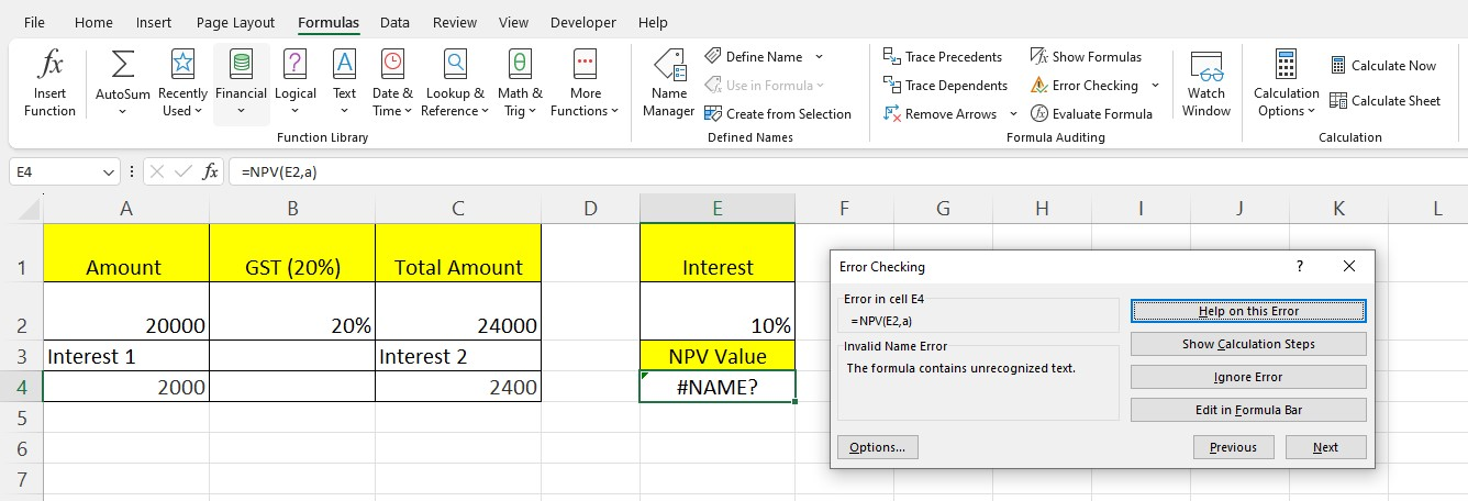
Check the following points of the Error Checking window:

• The left side of the window will show you any mistakes. Our mistake was that the formula had words that it needed to recognize.

• If you have an error, the "Help on this error" option will take you to a Microsoft page with instructions on how to fix it.

• The "Show Calculation Steps" option lets you see how you calculated the formula. It shows a dialog box with all the steps.

• If you click "Ignore Error," Excel will close the box. If you open the box again, it will ignore this error.

• The "Edit in Formula Bar" option got you to the cell's formula. You can make changes to the formula in this space.

Features of Excel Auditing Tools

• Formula Auditing helps to easily check the parts of a formula, like what charts, pivot tables, and form controls it uses. It also looks at validation for the formula.

• Formula Auditing is a tool that helps you check if your Excel worksheet has any problems. It can quickly show if there are any circular references.

• It is helpful to find mistakes quickly.

• Using a workbook will help you figure things out faster and make finding mistakes in your math equations easier.

• Formula Auditing involves checking if the numbers in different columns are correct.

• After completing calculations in your worksheet, you can use Formula Auditing to identify any errors.

Things to Remember when Auditing Formulas in Excel

• You can also see the dates as numbers if you click the "Show Formulas" option.

• To check if an Excel formula is correct, press the "F9" key.

• Excel will display an error message if there are no "Trace Precedents" in the cell.

• The Trace Dependents of a cell ensure that the formula in another cell references the cell; otherwise, an error message will appear.

Final Thoughts on Auditing Formulas in Excel

Auditing formulas in Excel is crucial to keeping your data consistent and accurate.

With the features that come with this program, you can identify any problems or errors that might exist in a formula or set of formulas quicker than ever before.

Visit Simple Sheets for more easy-to-follow Excel guides and financial model examples, and remember to visit the related templates section of this blog post.

For the most straightforward Excel video tutorials, subscribe to Simple Sheets on YouTube!

Frequently Asked Questions on Auditing Formulas in Excel

How do you see what formula evaluates in Excel?

Click Evaluate to check the value of the underlined reference. The result of the evaluation will appear in italics.

Why is the Excel formula not showing results?

Click on Formulas and Show Formulas to switch between displaying formulas and results.

Which tool can you use to find the cells that a formula is using?

Click the Trace Dependents button to see which cells connect to the active cell. You will see a blue arrow linking the active cell and other related cells.

Related Templates

Warehouse Management System Excel Template

Tender Management Analysis Excel Template

Internal Audit Evaluation Excel Template