How to Find Circular References in Excel

How often have you worked in Excel and realized something is wrong because the data doesn't make sense? For example, you might have two columns of numbers that add up to more than 100%. Often, you will get a circular reference warning but have no idea what it means. This happens when there is a circular reference somewhere in your spreadsheet. Fortunately, it's easy to find these errors--and this blog post will show you how!

What are Circular References?

Circular References are a standard error in Microsoft Excel, especially when dealing with extended, complex functions and formulas. A circular reference occurs whenever the cell reference in a recipe you placed inside a workbook becomes a direct or indirect reference. When the Excel sheet runs the formula, it does so in an endless loop. The error-checking function built into your Excel sheet helps stop your computer from eating itself and makes it easy to find circular references in your worksheet. 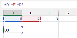In this example, the formula in Cell Address D3 directly references itself. This is also aptly called a direct circular reference. This Error isn't standard among seasoned Excel users, but anyone can fall victim to it. 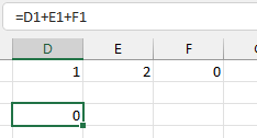The second kind of circular reference is called an indirect circular reference. In this example, we referenced the correct cell; no more referencing its cell nonsense, but it still returns the wrong answer. This is because cell address F1 contains a cell reference that references cell address D3. 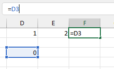Effectively, the cell addresses the D3 formula and refers to itself indirectly, causing you to create an indirect circular reference. We can see how this can pose a problem because it alters the results of your computations which could have a huge impact depending on the kind of work that you do. You only see the circular reference warning message window on the first instance of committing a circular reference error. So how can we identify, fix, and prevent circular references in Microsoft Excel?

Examples of Circular References

-A cell is referencing itself. In this case, the formula =SUM(B12) would be in B11, and the result of that calculation is added back to B12, making a loop. -Two cells with formulas referencing each other (a 'loop'). These often happen when you copy a range of cells and then paste them into another location on your spreadsheet - two rows will end up pasting into one row, but they still have their original relationships, so it looks like there are loops. For example, SUM(D45) in D44 will only sum values from column C if total sales for quarter Q are greater than or equal to 500000! A similar situation happens when copying columns. For example, if you have a column of unique values and copy it and then paste it to another area on your spreadsheet, the formulas in cells A11:A30 will not work as expected because they will be referencing different rows. If you program in Python, you may also experience circular references. This is a common problem if you have two variables that reference each other, such as def hello(name): print('Hello' + name) hello("Bob") In this case, the function will never return because it prints out "Hello" and does not exist. The variable name always points to itself, so there is no way for the program flow to continue. Circular references are very similar in Excel - we need to find them before they cause significant problems! - How do circular references happen? When copying rows or columns of data from one area on your spreadsheet into another, some cells might end up referencing themselves (rather than any external cell). Here are examples of how circular references can have real-life implications for your spreadsheets. 1) We have a budget of $1000 In this case, the budget will always be $1000 because it's referencing itself. The total amount spent will never change, so your spreadsheet is inaccurate. 2) When transferring funds between accounts in Quicken, if there are any cells with circular references on either side of the transfer (cells that refer to each other), you'll get an error message saying, "Cannot find referent for cell X." This means that these cells cannot both show new data without breaking their connection to themselves. To avoid errors when transferring funds in Quicken or Excel: keep track of which rows/columns contain circular references and don't try to edit or enter data in those cells.

How to Find Circular References

Finding Circular References the Old School (Hard) Way

This method would involve a bit of the hacker man in you. You can use this method if you're trying to look for circular references in an older version of Microsoft Excel. -Select your data, click the "Formulas" tab, and press F12 to open the Visual Basic Editor. -On the left side of the screen, you'll see a list of all Excel formulas currently used in your spreadsheet. -Look for any cells with an asterisk (*) next to them - these represent circular references (cells dependent upon each other), so they will show when viewing relationships between cells. -Click on one of those cell names and follow it until it stops at another formula or column header name. This is the endless loop we were talking about. You have found your circular reference! Now delete this cell's formula by clicking anywhere inside its box, then pressing Delete from your keyboard!

Find Circular References in Excel the Easy Way

If you're running a newer version of Excel, such as the Office 365 version, you're equipped with an arsenal of tools that make it easy to find circular references in Excel. These built-in tools make finding circular references in Excel too easy.

Right in Your Face.

You will get a circular reference warning message on the first instance of committing a circular reference error. Microsoft Excel's error-checking utilities are always on the lookout for any time you're probably ruining your spreadsheet. So when you save a circular reference, Excel displays this error message. Once you see this, you can correct your mistake or, depending on how you want to structure your Excel workbook, enable iterative calculation.

What's Your Status?

Excel has a status bar like your favorite social media platforms! The status bar is located at the bottom of your Excel Workbook. The status bar in Excel displays a few essential details, such as the workbook status; if you've selected some cells, you also get the average, count, and sum. Most importantly, it tells you you have circular references in the workbook. It even tells you the cell address where the circular reference is located. Just note that the status bar only shows one circular concern per sheet. In our simple example, only one circular reference is present. You can use the status bar for various uses, even for matters other than circular references.

The Formulas Tab is the Secret to Successful Calculation.

Depending on the nature of your work, you may or may not frequent the Formulas tab. Who will you call if you need help with your circular reference or any error? The Formulas tab! Most of Excel's error-checking tools are in the Formula Auditing Group. The first error-checking tool in the Formula Auditing Group that is probably the most useful is... well... the Error Checking tool! 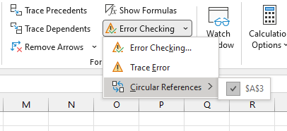You can easily click on it, and in the drop-down menu, select Circular References, which shows which cells contain circular references. Error Checking can also do a bunch of other cool tricks, like checking the entire worksheet for errors, and if you've got a selected cell address that you know has a mistake, you can trace the Error. You can do this for all the circular references in your Excel Workbook. This will also cover the hidden circular references in your Excel Workbook.

Tracing Precedents.

The Trace Precedents tool is another excellent tool in the Formulas tab > Formula Auditing Group. As the name suggests, this tool traces the different cells that precede or make up the values in a cell. 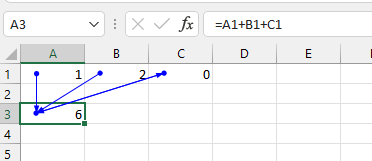We select the cell address, then hit the Trace Precedents button. The Trace Precedents tool adds arrows that point towards and away from the selected cell. The circles show the source, and the arrows indicate where they are directed. In this example, we can visibly see the circular reference. We can see in cell C3 that it's pointing towards cell A3, but at the same time, cell A3 also points toward cell C3. If we inspect cell C3 and check the formula bar, we'll see that cell C3 referenced cell A3 which is why there is a circular reference. 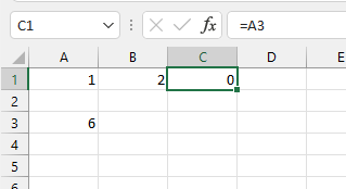In this simple example, we can also see how circular references can cause you to calculate incorrectly, which is always wrong.

Trace Dependents.

Trace Dependents do what Trace Precedent does but backward. While Trace Precedents let you know which cells precede the computations in that cell so you can investigate the different inputs to that formula, Trace Dependents let you know which procedures or cells depend on the cell/cells you selected. 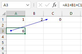In the above example, when we select cell A3 and click Trace Dependents, we can see which cells depend on cell A3. Cell C1 depends on cell A3 and would return a circular reference should we reference cell C3 later. Trace Precedents and Trace Dependents make spotting circular references easy, whether they're direct circular references or indirect circular references, because of their visual nature.

Take it Step-by-Step.

The Evaluate Formula tool is the last helpful tool you can use in the Formula Auditing Group to help spot circular references. You can select a cell containing the formula, giving you a play-by-play analysis of the procedure in question, and you can do this to all the recipes in the workbook.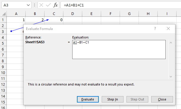

How To Remove Circular References

How do we deal with it now that we know how to find a circular reference in Excel? Unless you've got iterative calculations enabled on purpose, you might be inclined not to want to have a single circular reference issue in your sheet because it leads to calculating incorrectly. Generally, the only way to remove a circular reference is to fix the structure of your formulas. This is intrinsically a design error that should be prevented more than cured.

Due Diligence is Key.

Avoid circular references when possible - this helps you avoid errors because Excel will find any mistakes and alert you if there are any that it can detect. The status bar displays pertinent details and many more without asking. Remember that your mouse pointer picks up cell references when typing formulas. It's common to commit a plain circular reference error when typing in recipes using your mouse. Don't fret, though, because, as mentioned, a direct circular reference is more accessible to detect than an indirect circular reference. Remember not to reference the first cell by its cell to avoid a direct circular connection. Have a clear idea of how you want your Excel Function to be structured. This will take some time, but it yields dividends, especially when working with large spreadsheets and formulas. You can even draw the function out if you have to. This helps you avoid committing an indirect circular reference error. Create a table of contents with headers for each part of your spreadsheet; these headers should be text, not numbers, so the user knows what they're looking at without scanning through all the rows/columns on their screen. Use cell referencing instead of row/column references where appropriate (i.e., use A12 rather than B14) - this is helpful for users who may have different-sized monitors, as well as making sure your right and left-hand columns line up. Now that you know how to handle circular references, let's help you with your spreadsheets! Want more great tips on conquering Excel? Check out our Excel University or read about How to Show Changes or How to Compare Two Columns in Excel.