How To Convert Text to Numbers in Excel
Jan 10, 2025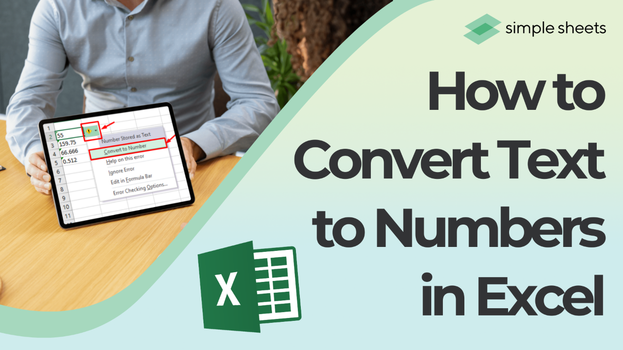
Last updated: August 19, 2026
Numbers stored as text sit left-aligned in the cell and are ignored by SUM. The fastest fix is to select the range, click the yellow warning icon, and choose Convert to Number. If no warning appears, copy an empty cell and use Paste Special, then Add, to force the conversion.
Have you tried calculating in Excel only to discover that your numbers act like text? It is a common issue that throws off your totals and leaves you scratching your head. Once you know which method matches your data, the fix takes seconds.
What is on this page
- Why do numbers turn into text in Excel?
- How do you tell if a number is stored as text?
- Which conversion method should you use?
- The five conversion methods, step by step
- How do you convert an entire column or sheet at once?
- What formula converts text to a number?
- Special cases: spaces, symbols, percentages and leading zeros
- Why is my conversion not working?
- How do you handle repeat imports with Power Query?
- How do you stop it happening again?
- Frequently asked questions
Get our free Excel formulas cheat sheet
Plus new tutorials and template drops. Enter your email and we'll send it over.

Why do numbers turn into text in Excel?
Knowing the cause matters, because it decides which fix will actually work. A number that is text because of a leading apostrophe needs a different fix from one that is text because of an invisible character glued to it.
| Cause | How it happens | Fix that works |
|---|---|---|
| Imported data | A CSV, a web page or a database export brings values in as text | Text to Columns, or Power Query |
| Leading apostrophe | Someone typed '1234 to stop Excel reformatting it |
Convert to Number, or Paste Special |
| Cell was Text first | The cell format was set to Text before the number was typed | Change format, then re-enter or use Paste Special |
| Hidden characters | A non-breaking space or a control character sits in the string | SUBSTITUTE, then TRIM, then VALUE |
| Wrong separators | The file uses a comma decimal, your Excel expects a full stop | NUMBERVALUE, or Power Query with a locale |
| Trailing minus | An accounting export writes negatives as 1234- |
Text to Columns with the trailing minus option |
The rule: if SUM returns zero over a column that clearly has numbers in it, the values are text. SUM does not error on text, it silently skips it.
Read more: How to Convert Date to Text in Excel.
How do you tell if a number is stored as text?
Four checks, from fastest to most definitive:
-
Alignment: numbers right-align by default, text left-aligns. A column of right-aligned values with a few left-aligned strays shows you exactly which cells are broken.
-
Green triangle: Excel flags text-based numbers with a small green triangle in the top-left corner of the cell.

-
ISTEXT: use =ISTEXT(cell_reference) to check a cell. TRUE means text. To count how many cells in a range are affected, use
=SUMPRODUCT(--ISTEXT(A1:A500)).
-
The status bar: select the range and look at the bottom right of the Excel window. If Excel shows Count but no Sum or Average, every selected value is text.
The rule: the status bar check is the most reliable, because it needs no formula and it works even when error checking has been switched off.
Which conversion method should you use?
Five methods do the same job, but they are not interchangeable. Pick from the row that matches your situation.
| Method | Best for | Works on multiple columns | Handles hidden characters |
|---|---|---|---|
| Convert to Number | Small ranges Excel has already flagged | Yes | No |
| Change cell format | Nothing on its own, see the warning below | Yes | No |
| Paste Special | Large ranges, and cells with no green triangle | Yes | No |
| Text to Columns | One column, and trailing minus signs | No, one column at a time | Partly |
| VALUE or NUMBERVALUE | Live data that keeps refreshing, and odd separators | Yes | Yes, when combined with SUBSTITUTE |
| Power Query | Imports you will repeat next month | Yes | Yes |
The rule: Paste Special is the default answer for a one-off cleanup of a big range. Power Query is the answer when the same messy file arrives again next month.
The five conversion methods, step by step
1. How do you use the Convert to Number option?
Excel's built-in error-checking tool is the quickest fix when your cells already display a green triangle, because Excel has spotted the problem for you.
Steps to convert:
-
Select the cells with the green triangle.

-
Click the error indicator (warning sign) that appears near the selected cells.

-
Choose Convert to Number from the dropdown menu.

Note: this suits small datasets. On a selection of many thousands of cells Excel processes them one at a time and can appear to freeze, so use Paste Special instead. Microsoft documents this route in its own guide to converting numbers stored as text to numbers.
2. Why does changing the cell format not convert the text?
This is the single most common false lead, so it is worth being precise about it. Selecting your cells, opening Format Cells and switching from Text to Number does not convert anything that is already in the cell. It only changes how future entries are displayed. The values stay text, the totals stay wrong, and nothing visible happens.
Changing the format is still a necessary first step, because a cell left on Text format will turn your converted numbers straight back into text. It just is not sufficient on its own.
Steps to convert:
-
Select the problematic cells.

-
Right-click and choose Format Cells from the context menu.

-
In the Format Cells dialog box, go to the Number tab.
-
Select Number or General, then click OK.
-
Now force the values to re-evaluate. Either double-click each cell and press Enter, or, far faster, run the Paste Special method in the next section across the whole range.

The rule: format controls display, not data type. Changing the format never converts existing text. Something has to make Excel re-evaluate the cell.
3. How do you convert text to numbers with Paste Special?
This forces Excel to re-evaluate every selected cell by performing a harmless arithmetic operation on it. It is the fastest method for large ranges and it works whether or not a green triangle is showing.
Steps to convert:
-
Type the number 1 in a blank cell and copy it with Ctrl and C.
-
Select the cells containing text-formatted numbers.

-
Right-click, choose Paste Special, and select Multiply in the Operation section.
-
Click OK to apply, then delete the helper cell containing the 1.

A variation that skips the helper cell entirely: copy any genuinely empty cell, select your range, then Paste Special and choose Add. Adding nothing changes no values but still forces the conversion, and you have nothing to clean up afterwards.
Note: multiplying by 1 does not change the numeric value, it only forces Excel to treat the content as a number. Watch for one side effect, which is that Paste Special can carry over the source cell's formatting. Use Paste Special, Values and Multiply together if the destination formatting matters.
4. How do you use Text to Columns to convert a column?
Text to Columns re-parses each cell exactly as if it had just been typed, which is why it works. It is the best option for a single column, and the only built-in option that handles trailing minus signs.
Steps to convert:
-
Highlight the column containing text strings. Click the column letter to take the whole column.
-
Go to the Data tab and click Text to Columns.

-
Select Delimited and click Next twice.

-
Under Column Data Format, choose General and click Finish.

On that final step, the Advanced button is where the useful settings hide. It lets you tell Excel which character is the decimal separator, which is the thousands separator, and whether negatives are written with a trailing minus. Setting those correctly solves most import problems in one pass.
Note: Text to Columns processes one column per run. For several columns, repeat it per column or use Paste Special instead.
Read more: How to Convert Formula to Text String in Excel.
5. How do you use the VALUE function?
The VALUE function reads a text string and returns the number it represents. Unlike the other methods it produces a new value in a new cell rather than changing the original, which makes it the right choice when the source data refreshes and you need the conversion to keep happening automatically.
Steps to convert:
-
In an adjacent column, enter
=VALUE(A1).
-
Double-click the fill handle to apply it down the column.
-
If you want to replace the originals, copy the results and use Paste Special, Values over the source column.
Note: VALUE returns the #VALUE! error if the string is not a recognisable number. Wrap it as =IFERROR(VALUE(A1),A1) to leave genuine text untouched instead of filling your column with errors.
How do you convert an entire column or sheet at once?
Most of the time the problem is not one cell, it is forty thousand. The method that scales is Paste Special, because it applies to any selection shape in a single pass.
To convert one whole column:
- Click the column letter to select the entire column, or click the first cell and press Ctrl, Shift and the Down arrow to select down to the last used row.
- Set the format to General first, through Home and then the Number Format dropdown. Leaving it on Text will undo your work.
- Copy an empty cell.
- Right-click the selection, choose Paste Special, select Add, and click OK.
To convert every text number on a sheet at once:
- Press Ctrl and A to select the used range.
- Set the format to General.
- Copy an empty cell, then Paste Special and Add.
Blank cells and real text labels are unaffected by adding zero, so a whole-sheet pass is safe as long as the sheet holds no formulas you would be overwriting. Paste Special overwrites formulas with their results, so run it on raw data, not on a calculated model.
The rule: set the format to General before the Paste Special, not after. Converting into a column still formatted as Text puts you straight back where you started.
What formula converts text to a number?
Four formula options, in increasing order of power:
| Formula | What it does | Use it when |
|---|---|---|
=A1+0 |
Adds zero, forcing numeric evaluation | You want the shortest possible formula |
=--A1 |
The double unary, negates twice | Inside SUMPRODUCT and array formulas |
=VALUE(A1) |
Parses the string using your regional settings | Standard imports that match your locale |
=NUMBERVALUE(A1,",",".") |
Parses using separators you specify | A file uses different separators from your Excel |
NUMBERVALUE is the one most people have never met, and it solves a problem the others cannot. If a European or Latin American export writes one thousand two hundred and thirty four point five six as 1.234,56, VALUE will either error or return the wrong figure on an English-language Excel. NUMBERVALUE lets you state the decimal separator and the group separator explicitly, so =NUMBERVALUE(A1,",",".") reads it correctly regardless of your regional settings.
The rule: use VALUE when the file matches your locale and NUMBERVALUE when it does not. Guessing between them is the reason imported European data so often lands off by a factor of a thousand.
Special cases: spaces, symbols, percentages and leading zeros
When the standard methods run and nothing changes, the cell almost always contains something you cannot see.
How do you remove leading and trailing spaces?
Spaces at either end stop Excel recognising the number. TRIM removes them.
-
In an adjacent cell, type
=TRIM(A1). -
Fill the formula down the column.
-
Copy the results, then right-click, choose Paste Special and select Values.
Why does TRIM not fix my data?
Because TRIM only removes the ordinary space, character 32. Data copied from a web page or a PDF very often contains the non-breaking space, character 160, which looks identical on screen and which both TRIM and CLEAN leave in place. This one character is behind a large share of conversions that appear to do nothing at all.
The fix is to substitute it out first:
-
=VALUE(TRIM(SUBSTITUTE(A1,CHAR(160),"")))handles the non-breaking space, then ordinary spaces, then converts. -
To confirm that is your problem before you fix it, check the length with
=LEN(A1). If a cell showing 1234 reports a length of 5, there is an invisible character in there.
How do you remove non-printable characters?
Imported text can carry control characters. The CLEAN function removes characters 0 to 31.
-
In a blank column, type
=CLEAN(A1). -
Fill down, then copy and paste back as values.
Pro tip: the belt-and-braces version that handles all three problems at once is =VALUE(TRIM(CLEAN(SUBSTITUTE(A1,CHAR(160),"")))).
How do you handle currency symbols and thousands separators?
VALUE copes with currency symbols and separators that match your regional settings, so =VALUE("$1,234.56") returns 1234.56 on a US English Excel. When the symbol does not match your locale, strip it first with =VALUE(SUBSTITUTE(SUBSTITUTE(A1,"$",""),",","")).
How do you convert a percentage stored as text?
VALUE understands the percent sign, so =VALUE("50%") returns 0.5. Remember that Excel stores 50 percent as the number 0.5 and uses the percentage cell format to display it as 50%. If you want the literal number 50 instead, use =VALUE(SUBSTITUTE(A1,"%","")).
How do you convert text to numbers without losing leading zeros?
You cannot keep them in the value itself. The number 007 and the number 7 are the same number, so any genuine conversion drops the zeros. That is correct behaviour, not a bug.
You have two options, and which one is right depends on what the data is:
-
If it is an identifier, such as a zip code, a product code or an account number, leave it as text. You are never going to add up zip codes, and text is the correct type for them.
-
If you need it numeric but displayed with padding, convert it and then apply a custom number format. Select the range, press Ctrl and 1, choose Custom, and enter
00000for a five-digit display. The underlying value stays a real number that arithmetic works on, while the cell still shows 00042.
For the full treatment of padding and formatting, see How to Add Leading Zeros in Microsoft Excel.
Read more: How to Convert Number to Date in Excel.
Why is my conversion not working?
When you have run a method and the numbers are still left-aligned, work down this table.
| Symptom | Likely cause | Fix |
|---|---|---|
| Nothing happens at all | The cells are still formatted as Text | Set the format to General first, then convert |
| No green triangle appears | Error checking is switched off | File, Options, Formulas, tick the rule for numbers formatted as text |
| Converts, then reverts on refresh | The source query re-imports as text each time | Set the column type in Power Query instead |
| VALUE returns #VALUE! | A hidden character, or a separator mismatch | Check LEN, then use SUBSTITUTE or NUMBERVALUE |
| Values off by a factor of 1000 | Decimal and group separators read the wrong way round | Use NUMBERVALUE with the separators stated |
| Negatives came through positive | A trailing minus sign, as in 1234- | Text to Columns, Advanced, tick trailing minus |
| Only some cells converted | Mixed causes in one column | Run TRIM and SUBSTITUTE first, then convert again |
| SUM still returns zero | The range is text-formatted, not the values | Select the range and check the status bar for a Sum |
The rule: if one method does nothing, do not just try another method. Find the hidden character first, because no conversion method will work until it is gone.
How do you handle repeat imports with Power Query?
If the same badly formatted file lands on your desk every week, converting it by hand every week is the wrong answer. Power Query records the cleanup once and replays it on each refresh.
- Select your data and go to Data, then From Table/Range.
- In the Power Query editor, right-click the problem column header.
- Choose Change Type, then Whole Number or Decimal Number.
- If the file uses foreign separators, choose Change Type, then Using Locale, and pick the country the file came from.
- Click Close & Load.
Next month, drop the new file in the same place and hit Refresh. The conversion runs itself.
How do you stop it happening again?
-
Set the format before you type: format cells as General or Number before entering data, never after.
-
Import rather than paste: use Data and then From Text/CSV instead of copying from a browser, so you can set column types during the import.
-
Use data validation: Excel's data validation tools can restrict a column to whole numbers or decimals and reject text outright.
-
Leave error checking on: the green triangle is genuinely useful. Turning it off to remove visual clutter means the next import fails silently.
Frequently asked questions
What is the fastest way to convert text to numbers in Excel?
Select the cells, click the error indicator next to the green triangle, and choose Convert to Number. For ranges larger than a few thousand cells, copy an empty cell and use Paste Special with the Add operation instead, which is much faster.
Why does changing the cell format to Number not convert my text?
Because the cell format controls display, not data type. Changing it affects future entries only, and leaves existing text untouched. You need to make Excel re-evaluate each cell, by re-entering the value, running Paste Special, or using Text to Columns.
How do I convert an entire column from text to numbers?
Click the column letter, set the format to General, copy an empty cell, then right-click and choose Paste Special with the Add operation. This converts the whole column in one pass and works on multiple columns at once, which Text to Columns does not.
What formula converts text to a number in Excel?
Use =VALUE(A1) for standard cases, or the shorthand =A1+0 and =--A1. When the file uses a comma decimal separator and your Excel expects a full stop, use =NUMBERVALUE(A1,",",".") to state the separators explicitly.
Why does my text still not convert after using TRIM?
TRIM only removes the standard space, character 32. Data copied from web pages often contains the non-breaking space, character 160, which TRIM and CLEAN both leave behind. Use =VALUE(TRIM(SUBSTITUTE(A1,CHAR(160),""))) instead, and check with =LEN(A1) whether the string is longer than it looks.
How do I convert text to numbers without losing leading zeros?
You cannot keep leading zeros inside a number, because 007 and 7 are the same value. Convert the cell, then apply a custom number format such as 00000 to display the padding. If the data is an identifier like a zip code, leave it as text instead.
How can I convert text to date format in Excel?
If your text is in a recognisable date format, such as 01/01/2023, use =DATEVALUE(A1) and then apply a date format to the result. DATEVALUE returns the serial number, so an unformatted cell shows a five-digit figure until you format it as a date.
How can I extract numbers from text in Excel?
Use the text functions LEFT, RIGHT and MID when the number sits in a predictable position. For a number mixed anywhere inside a string, =TEXT(MID(A1,ROW(INDIRECT("1:"&LEN(A1))),1)*1,"0") extracts the digits from A1.
Related Articles
How to Add Leading Zeros in Microsoft Excel
Want to Make Excel Work for You? Try out 5 Amazing Excel Templates & 5 Unique Lessons
We hate SPAM. We will never sell your information, for any reason.