How To Freeze a Column in Google Sheets
Feb 11, 2025
Did you know you can save time by freezing columns in Google Sheets?
Freezing a column in Google Sheets means locking it in place so that it remains visible as you scroll horizontally through your spreadsheet. This feature is great for extensive data sets, as it helps keep column headers, labels, or key identifiers in sight.
Read this article to learn how to freeze a column in Google Sheets like a pro.
Freezing a Column in Google Sheets (Step-by-Step Instructions)
Freezing a column in Google Sheets enhances your workflow and maintains data visibility. Here are step-by-step instructions on how to get it done:
-
Open your spreadsheet: Start by opening the spreadsheet where you want to freeze a column.
-
Select the column: Click on the lettered header of the column you wish to freeze.

-
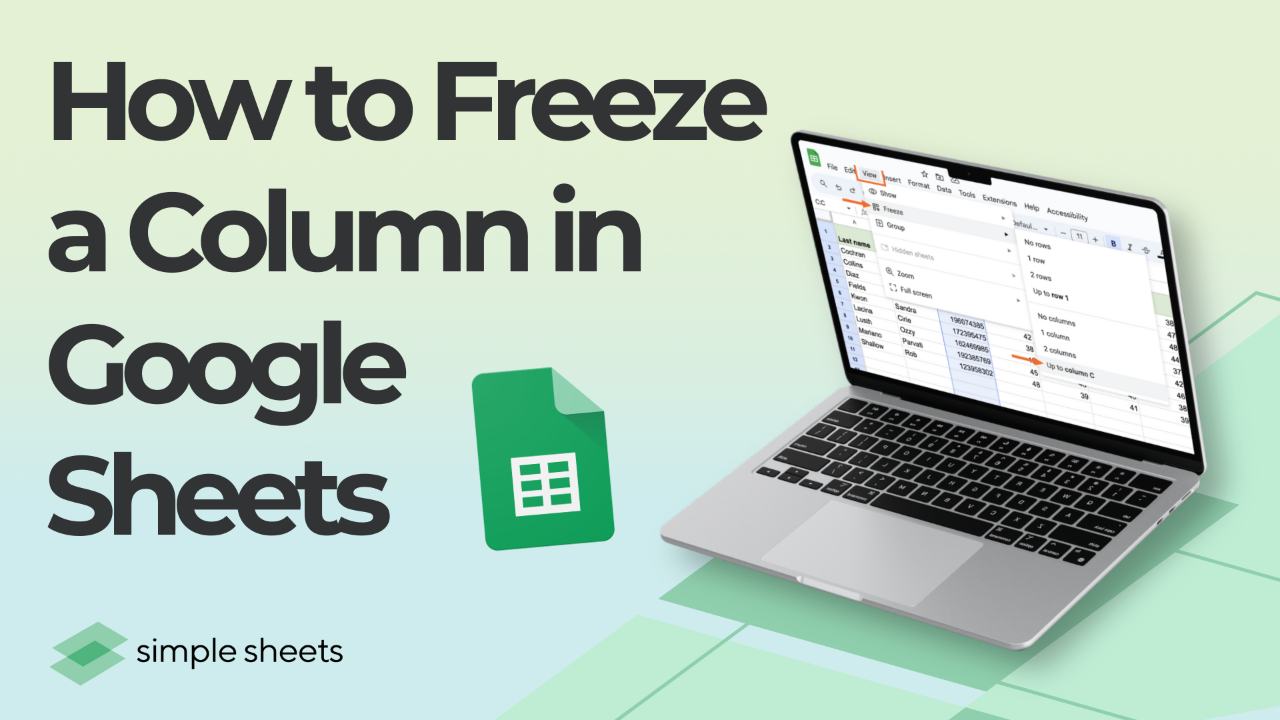
Access the View menu: At the top of the screen, click on the “View” tab.

-
Hover over 'Freeze': Hover over the “Freeze” option in the drop-down menu.
-
Choose the freezing option: Select “Up to current column” to freeze the currently selected cell or column.

Read more: How to Freeze Top Row and First Column in Excel.
Freezing multiple columns.
You may have a dataset that requires keeping two or more columns (e.g., "Name" and "Department") visible. Google Sheets allows freezing up to 5 columns, but this depends on your screen size. Note that the columns must be contiguous (no skipping columns).
-
Select the column you want your freeze point. For example, to freeze Columns A and B, click Column B’s header (the "B" label).

-
Go to View > Freeze > Up to column [X] (e.g., “Up to column B”).

Alternative method using the drag-and-drop shortcut.
You can also freeze rows and columns in Google Sheets using the drag-and-drop method. It is faster and easier to use:
-
Locate the thick gray line in the top-left corner of the sheet, right above the row numbers and next to the column letters.

-
Click and drag the gray line to the right, placing it after the column you want to freeze.

How To Freeze Columns on Mobile Devices
If you love working on your spreadsheets on the go, you should be pleased to know you can freeze columns on your mobile devices. We have explained how to freeze columns in Google Sheets on both Android and iOS devices below:
For Android:
-
Open the Google Sheets app.
-
Navigate to your spreadsheet.
-
Tap and hold the column letter you want to freeze.
-
Tap the three vertical dots that appear in the top-right corner.
-
Select Freeze from the options.
For iOS:
-
Launch the Google Sheets app.
-
Open your desired spreadsheet.
-
Tap the letter header of the column you want to freeze.
-
From the menu that appears, select Freeze.
How to Unfreeze Columns in Google Sheets
To unfreeze columns in Google Sheets, follow these simple steps:
-
Go to the View menu: Click “View” in the top menu bar.
-
Select Freeze: Hover over “Freeze” in the dropdown menu.
-
Unfreeze columns: You’ll see options like “No columns” or “No rows.” Click on “No columns” to unfreeze any columns that are currently locked in place.

-
Verify: Scroll through your sheet to confirm that the columns are free to move as you scroll horizontally.
Final Thoughts
Using the freeze feature in Google Sheets improves data management, particularly when handling large datasets. It allows you to keep crucial columns visible while scrolling. Apply the steps outlined above to streamline your workflow and get the most out of your Google Sheets experience.
For more easy-to-follow Excel guides and the latest Excel Templates, visit Simple Sheets and the related articles section of this blog post.
Subscribe to Simple Sheets on YouTube for the most straightforward Excel video tutorials!
FAQ
How can I freeze the first column in Google Sheets?
Follow these steps to freeze the first column in your sheet:
-
Open your Google Sheet.
-
Click View in the top menu bar.
-
Hover over Freeze in the dropdown.
-
Select 1 column.
How can I freeze multiple rows in Google Sheets?
To freeze multiple rows in Google Sheets:
-
Open your sheet and select the row below the last row you want to freeze.
-
Click on “View” in the top menu.
-
Hover over “Freeze” and choose “Up to current row (X),” where X is the selected row number.
How can I unfreeze rows in Google Sheets?
To unfreeze rows in Google Sheets:
-
Click on “View” in the top menu.
-
Hover over “Freeze” in the dropdown.
-
Select “No rows” to unfreeze all frozen rows.
Related Articles
How to Change Cell Size in Google Sheets
Want to Make Excel Work for You? Try out 5 Amazing Excel Templates & 5 Unique Lessons
We hate SPAM. We will never sell your information, for any reason.


