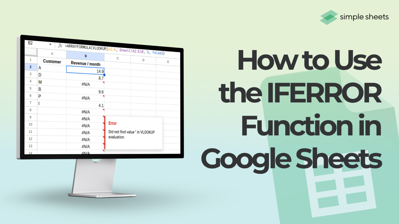
How To Use IFERROR in Google Sheets
Nov 18, 2024
It is almost inevitable not to encounter errors when using spreadsheets.
Whether a division by zero or a failed lookup, error messages like #DIV/0! or #N/A can disrupt your workflow. Fortunately, Google Sheets offers a function to handle these issues: IFERROR.
In this article, we’ll explore how to use the IFERROR function effectively and discuss how AI can help you with it.
What Is the IFERROR Function in Google Sheets?
The IFERROR function in Google Sheets is a built-in function designed to handle errors in your formulas. Instead of showing a standard error message like #DIV/0! or #N/A, the IFERROR function lets you replace these errors with a custom value or message. This makes your spreadsheets cleaner and easier to understand, especially when sharing with others.
IFERROR Formula: =IFERROR(value, [value_if_error])
-
value: The formula or expression to evaluate.
-
value_if_error: The value or message to return if the formula results in an error.
How does it work?
The IFERROR function evaluates the given value. If the result of value is an error, it returns the value_if_error message. If there’s no error, it simply returns the result of the value.
Errors it can handle.
The IF ERROR function can catch and replace these common Google Sheets errors:
-
#DIV/0!: Division by zero.
-
#N/A: Value not available (common in lookup functions).
-
#REF!: Invalid cell reference.
-
#VALUE!: Incorrect data type.
-
#NAME?: Misspelled function or named range.
-
#NUM!: Invalid numeric operation.
How To Use IFERROR Google Sheets
Now, let's show you how to use IFERROR in Google Sheets. Here are some practical applications of the function:
1. #DIV/0! (Division by zero).
This error occurs when a formula attempts to divide a number by zero or by a blank cell.
-
Example: =A1/0
-
Using IFERROR: =IFERROR(A1/B1, "Invalid Division")
If B1 is zero or empty, it will return "Invalid Division" instead of the error value #DIV/0!

2. #N/A (Value not available).
This happens when lookup functions like VLOOKUP or HLOOKUP can’t find a matching value.
-
Example: =VLOOKUP("Apple", A2:B5, 2, FALSE) (if "Apple" isn’t in column A).
-
Using IFERROR: =IFERROR(VLOOKUP("Apple", A2:B5, 2, FALSE), "Product Not Found")
The function returns "Product Not Found" instead of #N/A.

3. #REF! (Invalid cell reference).
The invalid cell reference error is triggered when a formula references a deleted or moved cell.
-
Example: =A1+B1 (if column A is deleted).
-
Using IFERROR: =IFERROR(A1+B1, "Reference Error")
The function displays "Reference Error" instead of #REF!.
Original sheet:
After deleting the first column:

4. #VALUE! (Wrong data type).
The #VALUE error typically occurs when a formula uses incompatible data types, like text in a mathematical calculation.
-
Example: ="text"/2
-
Using IFERROR: =IFERROR("text"/2, "Invalid Input")
This returns "Invalid Input" instead of #VALUE!.

5. #NAME? (Unrecognized function or range).
Results from a misspelled function name or undefined named range.
-
Example: =SUMM(A1:A10) (instead of =SUM).
-
Using IFERROR: =IFERROR(SUMM(A1:A10), "Name Error")
The IFERROR formula displays "Name Error" instead of #NAME?

6. #NUM! (Invalid numeric operation).
Triggered by an invalid calculation, such as taking the square root of a negative number.
-
Example: =SQRT(-1)
-
Using IFERROR: =IFERROR(SQRT(-1), "Invalid Number")
The formula returns "Invalid Number" instead of #NUM!.

Final Thoughts on "How To Use IFERROR in Google Sheets"
The IFERROR function is great for managing errors in Google Sheets. It helps you maintain clean and professional spreadsheets. By replacing confusing error messages with meaningful values, it improves the usability and clarity of your data.
For more easy-to-follow Excel guides and the latest Excel Templates, visit Simple Sheets and the related articles section of this blog post.
Subscribe to Simple Sheets on YouTube for the most straightforward Excel video tutorials!
FAQ on "How To Use IFERROR in Google Sheets"
1. What does the IFERROR function do in Google Sheets?
The IFERROR function replaces error messages like #DIV/0! or #N/A with a custom value or message. It ensures your spreadsheet remains clean and easy to understand.
2. Can IFERROR handle all types of errors in Google Sheets?
Yes, IFERROR can handle errors like #DIV/0!, #N/A, #REF!, #VALUE!, #NAME?, and #NUM!. It works universally across different types of formulas.
3. What happens if I don’t specify a value for value_if_error?
If you leave the value_if_error argument blank, IFERROR will return an empty cell for any error. This is useful when you want to hide errors without displaying a message.
Related Articles
How to Insert Bullets in Google Sheets
Want to Make Excel Work for You? Try out 5 Amazing Excel Templates & 5 Unique Lessons
We hate SPAM. We will never sell your information, for any reason.


