Definitive Guide: How to Make a Table in Google Sheets

Do you want to create a table in Google Sheets but need help figuring out where to start?

Knowing how to make a table in Google Sheets is simple. Moreover, having this skill can make your data look more professional.

You might question the necessity of creating a table in Google Sheets, even though the spreadsheet appears as one large table in its simplest form.

A Google Sheets table is much more than a collection of cells and is a must-have for presenting data. Today, we'll discuss this topic in detail.

Read on as we cover the following:

• Why make a Google Sheets table

• Steps to make a table in Google Sheets

• Steps to format a table in Google Sheets

• Final thoughts on how to make a table in Google Sheets

• Frequently asked questions about making a Google Sheets table

Why Make a Table in Google Sheets

You may think that making a table in Google Sheets is unnecessary, especially since spreadsheets look like blank tables.

However, you'd need to learn how to make a table in Google Sheets to present data in various ways. 

It organizes your data collection and allows you to add functions, colors, and filters.

Here are some reasons why you should make a table in Google Sheets:

Reason #1

A table in Google Sheets creates a way to store different types of data.

Moreover, it allows you to add column headings to your data. This way, you can easily add, retrieve, or review information. 

Reason #2

It is easy to see your data. Adding filters to your table lets you organize and view your data differently.

A table also makes presenting your data to others easier, ensuring that the information is organized and usable.

Reason #3

It is easy to track your work. Your table will have clear headings in the top row, giving you an organized worksheet.

Moreover, you can trace where you stop and monitor your progress and data input.

Besides, you can have multiple tables within Google Sheets. Once you learn how to do this, you can create several tables to organize all your data.

Steps to Make a Table in Google Sheets

Making a basic table in Google Sheets is quick and simple. Once you know the steps, you can format your table differently.

To make a table in Google Sheets, follow these steps:

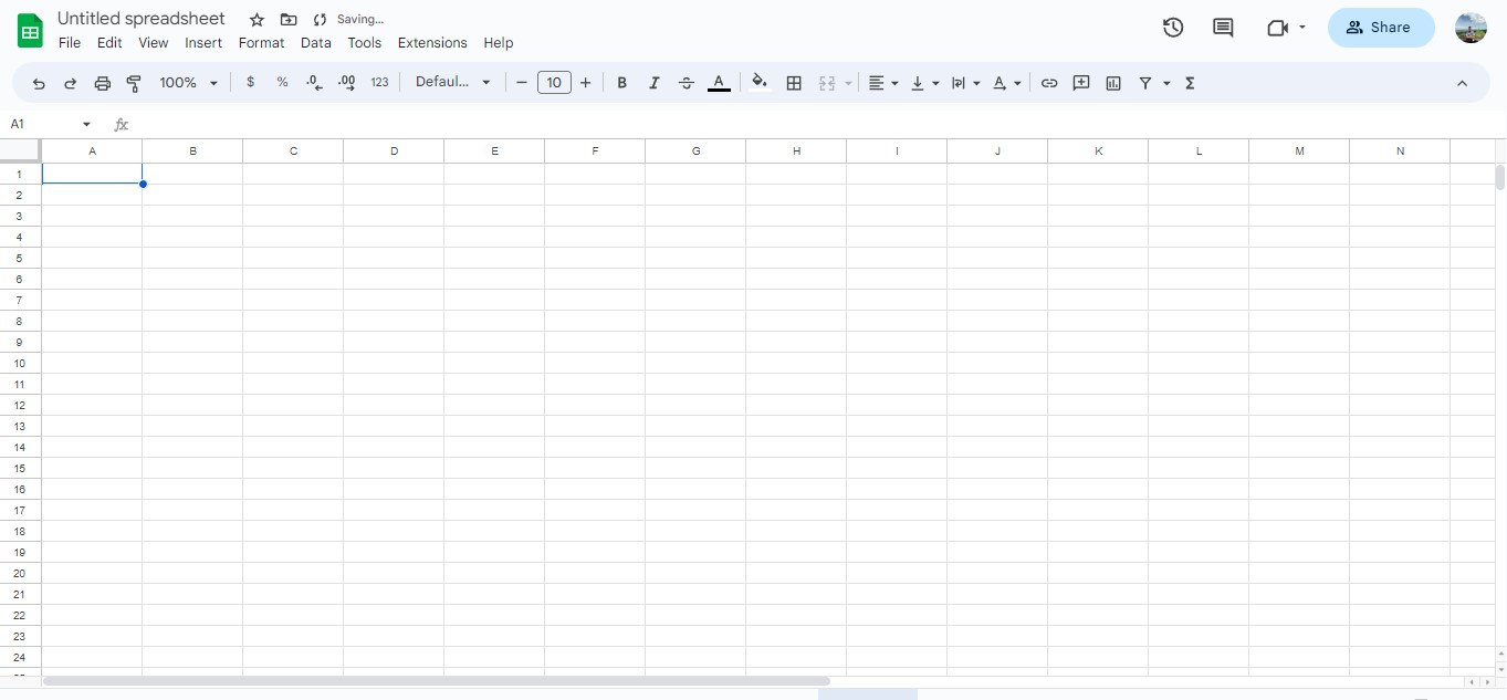
1. Launch Google Sheets and open your worksheet.

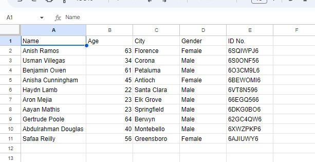
2. Make sure any data you want to put in your table has clear columns and, where relevant, row headings.

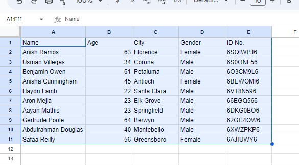
3. Select the data range (including the column headings) you want to include in your table.

4. In the toolbar of Google Sheets, click the Filter button.

5. Google Sheets will highlight your column headings in green and indicator arrows (small triangles) are next to your column headings.

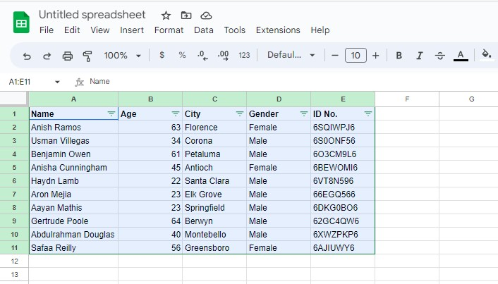
You now have a basic table in Google Sheets. From there, you can begin formatting your table.

Steps to Format a Table in Google Sheets

Now that you've learned to make a simple table in Google Sheets, you can customize your table.

You can do this by formatting a header row, aligning columns, organizing data, and adding colors.

Following the formatting tips and conditional formatting rules will elevate your table, making it look more professional. Moreover, it enables you to present data in different ways for analysis.

How to format a header row in Google Sheets

A header row is similar to a heading or title in a Word document. The first row of your spreadsheet is always the header row.

It provides a title for the data in your table.

Moreover, a header row as the first row at the top of your Google Sheets table enables you to label all the data within it.

To make your header row stand out and look professional, you can do the following:

• Use a different font for your header text to make it stand out from the rest of your Google Sheets table.

• Use a center-aligned header row to ensure the titles of your columns are center-aligned and the beginning or heading of the contents.

• Wrapping text is important as it means all the text in your header remains visible.

• Add a border. You can frame your header row to make it stand out. Moreover, you can have a border for the entire header row or individual cells.

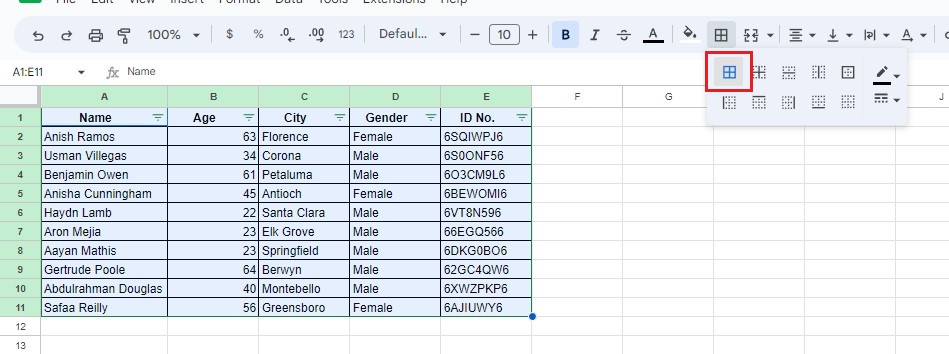
• Freeze the cells in the header row. By freezing the header row, it will remain visible as you scroll around the spreadsheet.

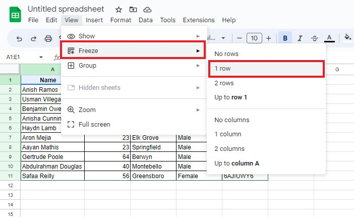
How to align columns in your table in Google Sheets

Another way to make your Google Sheets table look more professional, clear, and easy to read is to align the columns.

Alignment ensures that your columns are distant and work cohesively together.

To align the columns in your table:

1. Select the cell or desired cells to align, including, where relevant, the column header.

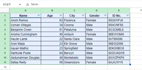
2. Go to your Google Sheets toolbar, click the Horizontal alignment menu, and select the Center option.

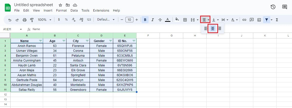
Aligned columns will polish your table formatting, making it clear and easy to read.

How to format data in Google Sheets

Using conditional formatting rules in Google Sheets, you can format your table so that its cells change color or text if they meet certain parameters.

Formatting data is more complex than the alignments and header rows, but it can elevate your Google Sheets table.

To format your data:

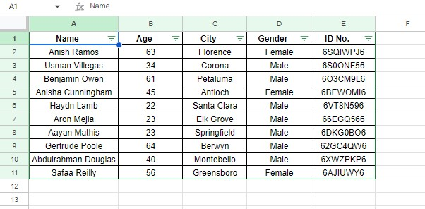
1. Select the cells you wish to format.

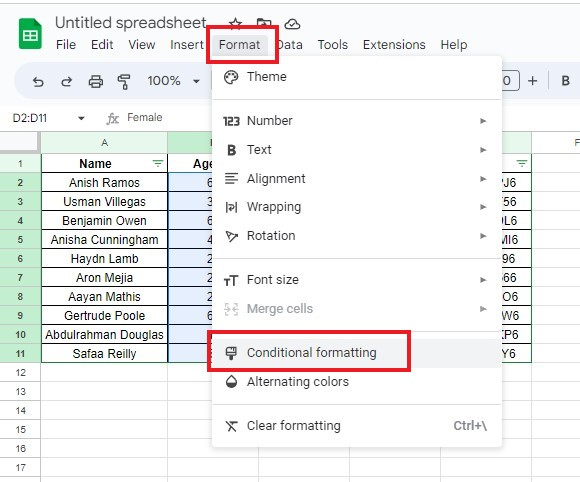
2. Click the Format menu and choose the Conditional Formatting option.

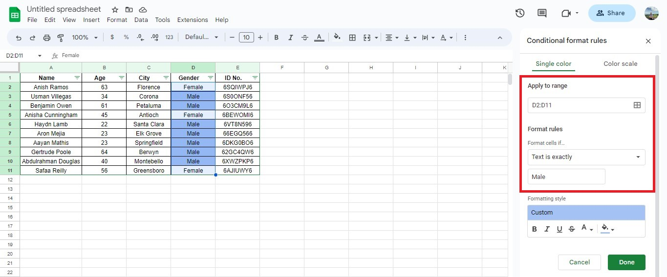
3. You can now create your rule. To do this, under Format Cells, choose the condition you want to trigger the rule.

4. Select Formatting Style, choose your desired conditions, and click the Done button.

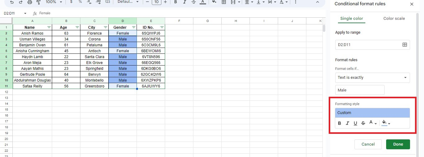
Now, whenever you enter data into your Google Spreadsheet that meets your set conditions, that cell will format to that style.

Once you start exploring it, there are many options for using conditional formatting in your Google Sheets table.

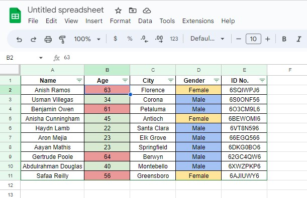
How to add colors to your table

Adding color to your Google Sheets table is quick and simple. What's more, customizing the colors can make your data stand out.

To add alternating colors to your table, simply:

1. Select the whole data in your table, including the header row.

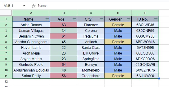
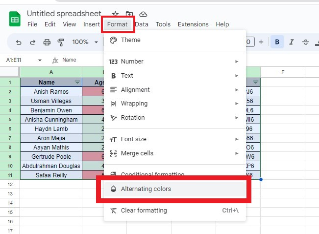
2. Go to the Format menu and select Alternating Colors.

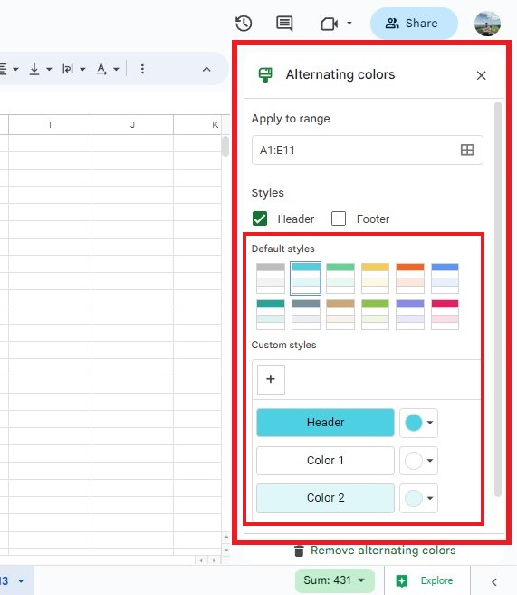
3. A dialog box will appear in a sidebar. You can choose your color options in this dialog box. Moreover, you can select either pre-programmed alternating colors or create your alternating colors.

4. Once you have made this selection, the highlighted rows will turn into those colors.

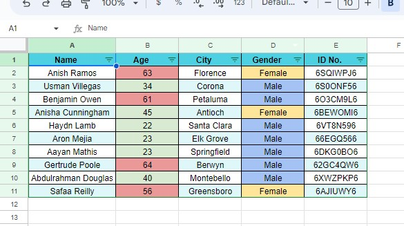
After that, all the data you add to your table will also take on those alternating colors.

Final Thoughts on How to Make a Table in Google Sheets

Making a table in Google Sheets is incredibly simple and flexible.

No matter your skill level or design sensibilities, you should follow these instructions to easily create a beautiful and effective table.

Visit Simple Sheets for more easy-to-follow guides and examples, and remember to read the related articles section of this blog post.

For the most straightforward Excel video tutorials, subscribe to Simple Sheets on YouTube!

Frequently Asked Questions About Google Sheets Tables

Can I add formulas to a Google Sheets table?

Absolutely! You can add formulas to any cell within a Google Sheets table. Use functions like SUM, AVERAGE, COUNT, etc., to perform calculations based on the data in the table.

How do I remove a table in Google Sheets?

To remove a table in Google Sheets, follow the steps below:

1. Select any cell within the table, then go to the Format menu.

2. Click on the table and select Delete Table from the drop-down menu.

Google Sheets will remove the table formatting, but the data will remain intact.

Can a table of contents be created for multiple sheets in Google Sheets?

To create a table of contents for multiple sheets on Google Sheets, go to the Insert menu and select Table of Contents. After clicking on it, a sidebar will select the sheets you want to add to the table of contents.

Related Articles

Creating a Monthly Budget Template in Google Sheets: Everything You Need to Know

How to Remove Duplicates in Google Sheets Without Using Apps Script

The Best Google Sheet Add-Ons That Can Make Your Life Easier