Remove Characters From the Left in Excel
Oct 29, 2024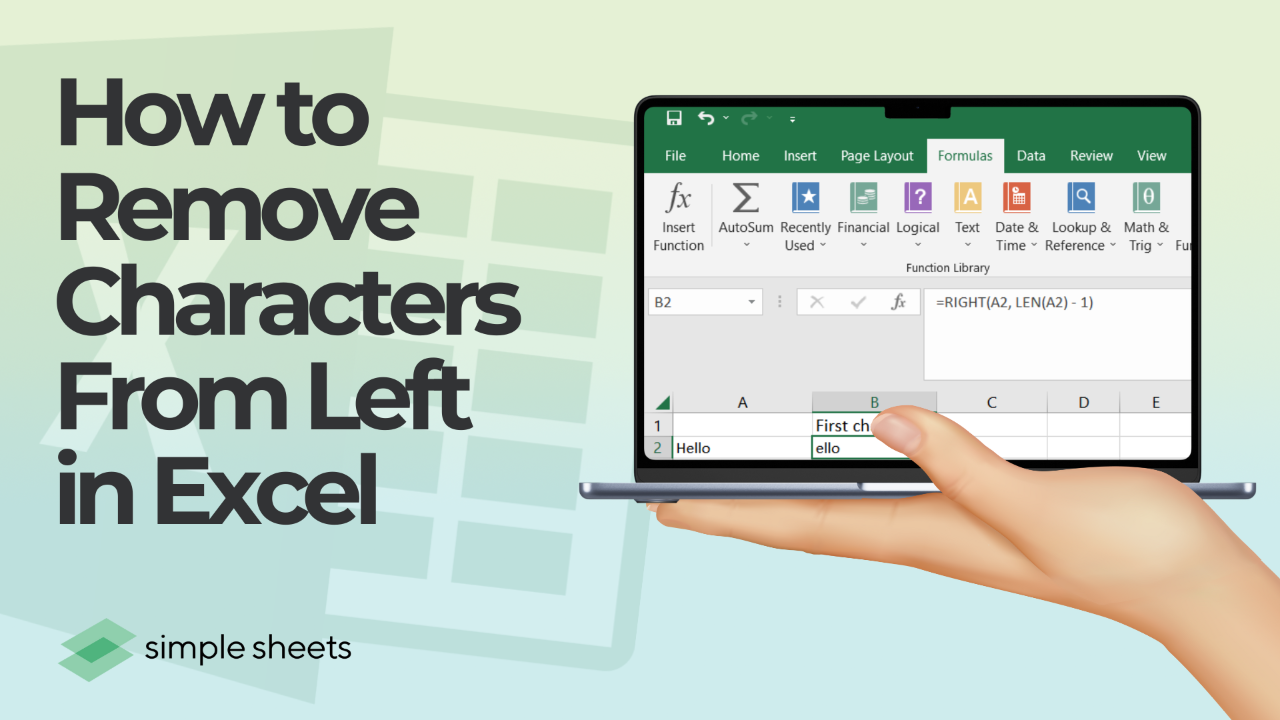
The short answer
To remove a fixed number of characters from the left in Excel, use =RIGHT(A1, LEN(A1)-n), where n is how many characters to strip. To remove a variable number, cut at a delimiter instead with =TEXTAFTER(A1, "-") in Microsoft 365, or =MID(A1, FIND("-", A1)+1, LEN(A1)) in older versions.
Last updated: August 18, 2026.
On this page
- Which method to use: fixed count vs. variable count
- Removing a fixed number of characters (RIGHT, REPLACE, MID)
- Removing a variable number of characters with FIND or SEARCH
- Removing everything before a character or delimiter
- Removing leading zeros specifically
- Removing leading spaces and non-printing characters
- The no-formula routes: Flash Fill and Text to Columns
- Power Query for cleanup you have to repeat
- Removing characters from the right instead
- Stripping letters or numbers rather than a position
- Getting AI to write the formula or the VBA
- Why your formula is returning an error
- Frequently asked questions
Get our free Excel formulas cheat sheet
Plus new tutorials and template drops. Enter your email and we'll send it over.
Do you need to clean up unwanted characters from the start of a cell in Excel?
Exported data almost never arrives clean. Product codes come prefixed with a vendor ID. Phone numbers arrive with a country code welded on. Account references land as CUST-00841 when the system downstream only wants 00841. Whether you are trimming extra spaces or removing specific text, you need to get your data right before anything else works.
This guide covers every route: the formulas for a fixed number of characters, the formulas for a variable number, the delimiter methods, the two no-formula options, and Power Query for when the same mess arrives every Monday. New to Excel functions? Start with the comparison table below and pick the row that matches your data.

Which method should you use to remove characters from the left?
Almost every wrong answer to this question comes from the same mistake: using a fixed-count formula on data where the count is not actually fixed. Find your situation in the first column.
| Your situation | Method | Formula | Watch out for |
|---|---|---|---|
| Fixed count. Always the same number of characters, e.g. always 4 | RIGHT with LEN | =RIGHT(A1, LEN(A1)-4) | Returns #VALUE! if any cell is shorter than 4 characters |
| Fixed count, and you prefer stating the position | REPLACE | =REPLACE(A1, 1, 4, "") | Never errors on short strings, it just returns an empty result |
| Fixed count, keeping everything from a set position on | MID | =MID(A1, 5, LEN(A1)) | The start position is n+1, not n. Off-by-one is the classic error |
| Variable count, but there is a delimiter such as a dash, colon or space | TEXTAFTER (Microsoft 365) | =TEXTAFTER(A1, "-") | Not available in Excel 2021 or earlier |
| Variable count with a delimiter, older Excel | MID with FIND | =MID(A1, FIND("-", A1)+1, LEN(A1)) | FIND is case-sensitive. Use SEARCH if case varies |
| Variable count, delimiter appears more than once | TEXTAFTER with an instance number | =TEXTAFTER(A1, "-", 2) | Use -1 to cut after the last occurrence instead of the first |
| Leading zeros on what should be a number | Multiply by 1, or VALUE | =VALUE(A1) | Only if the result should genuinely be numeric |
| Leading spaces or invisible characters | TRIM with CLEAN | =TRIM(CLEAN(A1)) | Neither one touches CHAR(160), the web non-breaking space |
| One-off job, pattern is obvious, no formula wanted | Flash Fill | Type the first result, press Ctrl+E | Static output. It does not update when the source changes |
| Same cleanup every week on a new export | Power Query | Transform > Extract > Text After Delimiter | Setup takes ten minutes, then it is one refresh click forever |
Rule to remember: If you can count the characters to remove and the number never changes, use RIGHT with LEN. If the number changes row to row, stop counting and cut at the delimiter instead.
How do you remove a fixed number of characters from the left?
Three functions do this job. They give identical results on clean data and behave differently on messy data, which is the only reason to care which one you pick.
RIGHT with LEN
The most common approach. LEN counts the characters, you subtract the ones you want gone, and RIGHT keeps what is left.
Formula: =RIGHT(A1, LEN(A1) - 1)
- LEN(A1) calculates the total number of characters in the string within cell A1.
- Subtracting 1 removes the first character.
- RIGHT(A1, LEN(A1) - 1) extracts all characters from the right side, except the first one.
Example: with "Hello" in A1, =RIGHT(A1, LEN(A1) - 1) returns "ello".
Change the number to change how much comes off. To remove the first 4 characters, use =RIGHT(A1, LEN(A1) - 4). To remove the first 5, use =RIGHT(A1, LEN(A1) - 5). The pattern holds for any n.
Rule to remember: RIGHT with LEN breaks the moment a cell is shorter than the number you are subtracting. Wrap it as =IFERROR(RIGHT(A1, LEN(A1)-4), A1) so short rows pass through untouched instead of showing #VALUE!.
REPLACE
REPLACE removes characters from the left by replacing them with an empty string. It is the most readable of the three because you state the position and the count directly.
Formula: =REPLACE(A1, 1, X, "")
- A1: the cell containing the text.
- 1: the starting position, meaning start replacing at the first character.
- X: the number of characters you want to remove from the left.
- "": replaces the removed characters with nothing.
Example: with "12345Text" in A1, =REPLACE(A1, 1, 5, "") returns "Text".
REPLACE has one practical advantage over RIGHT with LEN: it does not error on short strings. Feed it a three-character cell and ask it to remove five, and it returns an empty string rather than #VALUE!. On imported data with inconsistent row lengths, that is often the behaviour you want.
MID
MID lets you specify the starting position of the substring you want to keep, which suits cases where you think in terms of "keep everything from character 6 onward".
Formula: =MID(A1, X+1, LEN(A1))
- X+1 tells Excel to start extracting from the position after the first X characters.
- LEN(A1) defines the total length of the string, ensuring it extracts everything after the removed characters.
Example: with "12345Text" in A1, =MID(A1, 6, LEN(A1)) returns "Text".
Note the 6, not the 5. To remove five characters you start at the sixth. That off-by-one is the single most common mistake with MID, and it is why the formula above is written as X+1.
How do you remove a variable number of characters using FIND or SEARCH?
This is where most real data lands. The prefix is not always the same length, so counting does not work. Instead you find a landmark inside the string and cut relative to it.
FIND returns the position of a character inside the text. Feed that position into MID or RIGHT and the formula adapts row by row.
Cut everything up to and including the first dash:
=MID(A1, FIND("-", A1) + 1, LEN(A1))
With CUST-00841 that returns 00841. With SUPPLIER-77 it returns 77. Different prefix lengths, same formula, no counting.
Cut everything up to the first space:
=MID(A1, FIND(" ", A1) + 1, LEN(A1))
This is how you strip a first name off "Sarah Mitchell" without knowing how long the first name is.
FIND vs. SEARCH
They take the same arguments and differ in two ways that matter:
- FIND is case-sensitive. FIND("a", "ABC") returns an error. SEARCH("a", "ABC") returns 1.
- SEARCH accepts wildcards. SEARCH("?-", A1) finds a dash preceded by any single character.
Use SEARCH by default on imported data, where you cannot trust the casing. Use FIND when case actually distinguishes what you are looking for. Our full walkthrough of the function is here: The Easiest Guide For FIND Function Excel.
Rule to remember: FIND and SEARCH return #VALUE! when the character is not present. Always wrap the whole thing: =IFERROR(MID(A1, FIND("-",A1)+1, LEN(A1)), A1). Rows without a dash then pass through unchanged instead of poisoning the column.
How do you remove everything before a specific character or delimiter?
In Microsoft 365 there is a purpose-built function for exactly this, and it replaces the MID and FIND combination entirely.
TEXTAFTER
Formula: =TEXTAFTER(A1, "-")
That is the whole thing. It returns everything after the first dash. No LEN, no FIND, no position arithmetic.
The third argument controls which occurrence to cut at, which is what makes it genuinely more capable than the older approach:
- =TEXTAFTER(A1, "-", 1) cuts after the first dash. This is the default.
- =TEXTAFTER(A1, "-", 2) cuts after the second dash. With AB-CD-EF that returns EF.
- =TEXTAFTER(A1, "-", -1) cuts after the last dash, counting from the end.
- =TEXTAFTER(A1, "-", 1, 1) makes the match case-insensitive.
- =TEXTAFTER(A1, "-", 1, 0, 1) returns the original text if the delimiter is missing, instead of an error. This one argument replaces the IFERROR wrapper.
Microsoft documents the full argument list on the TEXTAFTER function reference.
If you do not have TEXTAFTER
TEXTAFTER arrived with Microsoft 365 and is not in Excel 2021, 2019 or 2016. On those versions:
- First occurrence: =MID(A1, FIND("-", A1)+1, LEN(A1))
- Last occurrence: =TRIM(RIGHT(SUBSTITUTE(A1, "-", REPT(" ", 100)), 100))
That second formula looks strange and is a genuinely useful trick. SUBSTITUTE swaps every dash for 100 spaces, RIGHT grabs the last 100 characters, and TRIM cleans up the padding. What survives is everything after the final dash, whatever length it was.
Rule to remember: The REPT padding trick works on any delimiter and any string length under 100 characters. Raise the 100 to 255 if your data is long.
How do you remove leading zeros in Excel?
Leading zeros are a special case, because how you remove them depends on what the value actually is.
If the result should be a number
The zeros are only there because the cell is formatted as text. Convert it and they disappear on their own:
- =VALUE(A1) converts the text to a number. 00841 becomes 841.
- =A1*1 or =A1+0 does the same thing with less typing.
- Text to Columns with no changes: select the column, Data > Text to Columns, Next, Next, choose General, Finish. Excel re-evaluates every cell and drops the zeros in place, no helper column needed.
If the result should stay text
Product codes and account references are text that happens to look numeric. Converting them to numbers is destructive, because you cannot get 00841 back from 841 without knowing the original width. Strip only the zeros and keep it as text:
=MID(A1, FIND(LEFT(SUBSTITUTE(A1, "0", ""), 1), A1), LEN(A1))
That finds the first character that is not a zero and keeps everything from there. In Microsoft 365 there is a cleaner version:
=TEXTAFTER(A1, "0", -1)
which cuts after the last zero. Use this only when you know the zeros are all at the front, since a trailing or embedded zero will throw it off.
Going the other direction is a different job entirely: How to Add Leading Zeros in Microsoft Excel.
How do you remove leading spaces and non-printing characters?
When a formula that should work returns nothing useful, invisible characters are usually why. Three functions handle three different kinds of invisible.
| Problem | Function | What it removes |
|---|---|---|
| Leading, trailing and doubled spaces | =TRIM(A1) | All spaces at the ends, and any run of spaces inside reduced to one |
| Line breaks, tabs, control characters from a database or PDF export | =CLEAN(A1) | The first 32 non-printing ASCII characters |
| Copied from a web page and TRIM does nothing | =TRIM(SUBSTITUTE(A1, CHAR(160), " ")) | The non-breaking space, CHAR(160), which TRIM cannot see |
| All of the above at once | =TRIM(CLEAN(SUBSTITUTE(A1, CHAR(160), " "))) | The belt-and-braces version. Use this on anything pasted from a browser |
Rule to remember: If TRIM appears to do nothing, you have CHAR(160) rather than a normal space. Check with =CODE(LEFT(A1,1)). A result of 160 confirms it, 32 means an ordinary space.
More on the space-specific cases: Essential Steps To Remove Spaces in Excel and Excel: Remove Trailing Spaces.
How do you remove characters from the left without a formula?
Two options, and they suit different jobs.
Flash Fill
- In the column beside your data, type the result you want for the first row. If A2 holds CUST-00841, type 00841 in B2.
- Press Ctrl+E.
- Excel infers the pattern and fills the rest of the column.
Flash Fill handles patterns that would take a nested formula to express, and it is genuinely good at variable-length prefixes. Give it two examples rather than one if the first fill looks wrong.
The catch is that the output is static text. It does not update when the source data changes, and it does not survive a fresh export. Flash Fill is for one-off cleanups.
Text to Columns
Better when there is a clean delimiter and you want the pieces in separate columns anyway.
- Select the column. Go to Data > Text to Columns.
- Choose Delimited and click Next.
- Tick the delimiter, or type it into the Other box. Click Next.
- For any part you do not want, select that column in the preview and choose Do not import column (skip).
- Set the destination and click Finish.
Text to Columns overwrites the columns to the right of your data without warning, so insert blank columns first. Full walkthrough: Learn How to Split Cells in Excel.
How do you set up repeatable cleanup with Power Query?
If the same export arrives every week with the same prefix problem, stop rewriting formulas. Power Query records the steps once and replays them on every refresh.
- Select your data and go to Data > From Table/Range.
- In the Power Query Editor, click the column header to select it.
- Go to Transform > Extract.
- Choose Text After Delimiter and type your delimiter, or choose Text Range and set a start position to strip a fixed count.
- Click Close & Load.
Next week, paste the new export over the source table and click Refresh. Every transformation reruns in order. Power Query also handles the awkward cases well: it will strip a variable prefix, trim, clean, and change the data type in one pass, and it records each step so you can see and edit what happened.
Rule to remember: If you have cleaned the same file more than twice, the formula was the wrong tool. Ten minutes in Power Query pays for itself by the third refresh.
Start here if you have not used it: Mastering Power Query in Excel: A Guide for Beginners.
How do you remove characters from the right instead?
Same logic, mirrored. LEFT keeps the front of the string instead of the back.
- Remove the last character: =LEFT(A1, LEN(A1) - 1)
- Remove the last 4 characters: =LEFT(A1, LEN(A1) - 4)
- Remove everything after the last dash: =TEXTBEFORE(A1, "-", -1) in Microsoft 365
- Older Excel equivalent: =LEFT(A1, FIND("~", SUBSTITUTE(A1, "-", "~", LEN(A1)-LEN(SUBSTITUTE(A1,"-","")))) - 1)
TEXTBEFORE is the mirror of TEXTAFTER and takes the same arguments in the same order.
How do you remove letters or numbers rather than a position?
Sometimes the thing you want gone is not at a fixed position at all. It is every letter, or every digit, wherever it appears.
Keep only the numbers
In Microsoft 365, this dynamic array formula strips everything that is not a digit:
=TEXTJOIN("", TRUE, IFERROR(MID(A1, SEQUENCE(LEN(A1)), 1) * 1, ""))
It splits the string into individual characters, multiplies each by 1, discards anything that errors (which is every non-digit), and joins the survivors back together.
Keep only the letters
=TEXTJOIN("", TRUE, IF(ISERROR(MID(A1, SEQUENCE(LEN(A1)), 1) * 1), MID(A1, SEQUENCE(LEN(A1)), 1), ""))
The same idea inverted: keep the characters that fail the numeric test.
Remove one specific character everywhere
=SUBSTITUTE(A1, "-", "") removes every dash in the string, front, middle and end. Nest them to remove several: =SUBSTITUTE(SUBSTITUTE(A1, "-", ""), "/", ""). See How to Remove Dashes in Excel for the phone-number and SSN cases.
Rule to remember: SUBSTITUTE removes a character everywhere. REPLACE removes whatever sits at a position. Choosing the wrong one is why a formula that looks right gutted the middle of your data.
Can AI write the formula or the VBA for you?
You do not need to master Excel functions to remove characters from the left in your cells. With tools like ChatGPT and Perplexity AI, you can generate formulas or scripts based on your needs. It is a reasonable shortcut for a one-off, as long as you test the output before running it on real data.
Method 1: Asking for a formula
Step 1: Open ChatGPT or any AI tool you prefer.
Step 2: Use a prompt that names the cell and the count. For example: "Generate an Excel formula to remove the first 5 characters from cell A1."
Step 3: Copy the generated formula. For that prompt you will get =RIGHT(A1, LEN(A1) - 5), which calculates the length of the text in A1, subtracts 5, and returns the rest of the string. This is the same Excel formula covered above, arrived at faster.
Be specific about the awkward parts. If your prefix length varies, say so in the prompt, otherwise you will get a fixed-count formula that silently mangles half your rows.
Method 2: Using a VBA script
For more complex scenarios, you can ask AI to generate a VBA script to automate the task across many cells.
Prompt example: "Can you generate a VBA script that removes the first 3 characters from every cell in column A?"
You will get something like this:
Sub RemoveLeftChars()
Dim cell As Range
For Each cell In Range("A1:A100")
cell.Value = Right(cell.Value, Len(cell.Value) - 3)
Next cell
End Sub
This removes the first three characters from every cell in the range. You can modify the range and the number of characters as needed. Two warnings: VBA edits cells in place with no undo, so work on a copy, and this script will error on any cell shorter than three characters.
Read more: How to Open the VBA Editor.
Why is my formula returning an error?
#VALUE!
Either a cell is shorter than the number of characters you are removing, or FIND could not locate the delimiter in that row. Wrap the formula in IFERROR to see which rows are affected: =IFERROR(your_formula, "CHECK").
The formula returns the original text unchanged
The cell is formatted as Text, so Excel is displaying your formula rather than evaluating it. Change the cell format to General, then press F2 and Enter to re-enter it.
The result looks right but comparisons still fail
There are trailing spaces or a CHAR(160) hiding at the end. Wrap the result in TRIM, or use the combined cleanup formula from the section above.
#NAME?
Your Excel version does not have the function. TEXTAFTER, TEXTBEFORE, TEXTSPLIT and SEQUENCE are Microsoft 365 only. Use the MID and FIND alternatives given above.
The results disappear when I delete the original column
Your formulas still reference the deleted cells and now return #REF!. Convert the results to values before deleting anything: copy the results column, then paste as values. Full method: How To Remove Formula in Excel (While Keeping the Data).
Frequently asked questions
What is the formula to remove the first character in Excel?
=RIGHT(A1, LEN(A1)-1). It counts the characters, subtracts one, and keeps the rest from the right. =REPLACE(A1, 1, 1, "") does the same thing and does not error on empty cells.
How do I remove the first 4 characters in Excel?
Use =RIGHT(A1, LEN(A1)-4), or =REPLACE(A1, 1, 4, ""), or =MID(A1, 5, LEN(A1)). All three return the same result. MID needs 5 rather than 4 because you are naming the position to start from, not the count to remove.
How do I remove characters from the left when the number varies by row?
Do not count. Cut at a delimiter instead. Use =TEXTAFTER(A1, "-") in Microsoft 365, or =MID(A1, FIND("-", A1)+1, LEN(A1)) in older versions. Both adapt to whatever the prefix length happens to be.
How do I remove everything before a specific character?
=TEXTAFTER(A1, ":") returns everything after the first colon. Add a third argument to target a later occurrence, or -1 to cut after the last one. Without Microsoft 365, use =MID(A1, FIND(":", A1)+1, LEN(A1)).
How do I remove leading zeros without turning the value into a number?
Use =TEXTAFTER(A1, "0", -1) in Microsoft 365, or =MID(A1, FIND(LEFT(SUBSTITUTE(A1,"0",""),1), A1), LEN(A1)) in older versions. If the value should genuinely be numeric, =VALUE(A1) is simpler and drops the zeros automatically.
Why does TRIM not remove my leading spaces?
Because they are not spaces. Text copied from a web page usually contains CHAR(160), the non-breaking space, which TRIM ignores. Use =TRIM(SUBSTITUTE(A1, CHAR(160), " ")) instead. Confirm with =CODE(LEFT(A1,1)): 160 is the non-breaking space, 32 is a normal one.
Can I remove characters without a formula?
Yes. Type the desired result for the first row in the next column and press Ctrl+E to run Flash Fill. For repeatable cleanup on a file that arrives regularly, use Power Query: Data > From Table/Range, then Transform > Extract > Text After Delimiter.
Is TEXTAFTER available in my version of Excel?
Only in Microsoft 365 and Excel for the web. Excel 2021, 2019 and 2016 return #NAME? and need the MID with FIND combination instead.
Final thoughts
Removing characters from the left is one decision followed by one formula. If the count is fixed, use RIGHT with LEN and wrap it in IFERROR. If the count varies, stop counting and cut at a delimiter with TEXTAFTER or MID with FIND. If the same file arrives every week, build it once in Power Query and never think about it again.
Then convert the results to values before you delete the source column, or the whole thing collapses into #REF! errors.
For more easy-to-follow Excel guides and the latest Excel Templates, visit Simple Sheets and the related articles section of this blog post.
Subscribe to Simple Sheets on YouTube for the most straightforward Excel video tutorials!
Related Articles
How to Find Circular Reference in Excel Using AI
How to Freeze the Top Row and First Column in Excel
Want to Make Excel Work for You? Try out 5 Amazing Excel Templates & 5 Unique Lessons
We hate SPAM. We will never sell your information, for any reason.