How To Remove a VLOOKUP Formula In Excel
Mar 08, 2023
Do you need to remove a VLOOKUP formula in Excel without losing the results it produced?
Quick answer: Select the cells holding the VLOOKUP formulas, press CTRL+C to copy, then paste them straight back over the same selection using Paste Special and Values. Excel keeps every number and name the lookup returned and deletes only the formula behind it. The fastest keyboard route is CTRL+C, then CTRL+ALT+V, then V, then Enter.
Last updated: August 24, 2026
Get our free Excel formulas cheat sheet
Plus new tutorials and template drops. Enter your email and we'll send it over.
Read on as we cover the following:
New to the function itself, or trying to get one working rather than get rid of it? Start with our full guide to how to use VLOOKUP in Excel, which covers the syntax and the arguments in detail. This article is only about taking a finished VLOOKUP back out again.
What removing a VLOOKUP formula actually does
A VLOOKUP cell holds two things: the formula, written as =VLOOKUP(lookup_value, table_array, col_index_num, [range_lookup]), and the result that formula last produced. Removing the formula throws away the first and keeps the second. The cell stops being a live lookup and becomes an ordinary typed-in value.
Three reasons people do it:
-
To freeze a snapshot. Once the formula is gone, the value cannot change when the source table changes, gets re-sorted, or gets deleted.
-
To make the workbook lighter. Excel recalculates every live VLOOKUP whenever anything in the workbook changes. On a sheet with thousands of lookups that is the single biggest reason a file feels slow. Converting them to values removes that work entirely.
-
To send the file safely. A VLOOKUP that points at another workbook or a sheet you are not sending will break the moment it lands in someone else's inbox. Flattening it first means they see the numbers, not a wall of errors.
Rule: Removing a VLOOKUP formula does not make your results more accurate. It makes them permanent. If the underlying data was wrong, flattening it just locks the wrong answer in place. Check the numbers first.
These steps are not VLOOKUP specific either. If you searched for how to remove lookup in Excel, or you are working with HLOOKUP, XLOOKUP or an INDEX and MATCH pair, every method below behaves identically.
People search for this a dozen different ways: how to remove VLOOKUP formula in Excel, remove VLOOKUP formula in Excel and keep values, how to remove VLOOKUP in Excel, or how to delete VLOOKUP formula in Excel. Every one of them wants the same three seconds of work.
Five ways to remove a VLOOKUP formula, compared
| Situation | Method | Speed |
|---|---|---|
| A handful of cells you can see | Copy, then right-click and choose Values under Paste Options | Fastest by mouse |
| The same, without leaving the keyboard | CTRL+C, then CTRL+ALT+V, then V, then Enter | Fastest overall |
| You do not know which cells hold formulas | CTRL+G, Special, Formulas, then paste values | Two extra clicks, catches everything |
| The same layout across several worksheets | Group the sheets with Shift, then paste values | One pass for all sheets |
| You want to move the cells at the same time | Right-drag the selection, choose Copy Here as Values Only | No clipboard step |
| Hundreds of sheets, or you repeat this weekly | A VBA macro | One keypress once it is set up |
Method 1: Paste Values on a single sheet
This is the method almost everyone wants. It removes the formula and keeps the value, in place, in about three seconds.
-
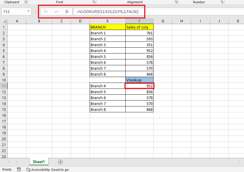
Locate the cells that contain the VLOOKUP formula. Click one and check the formula bar to confirm.
-
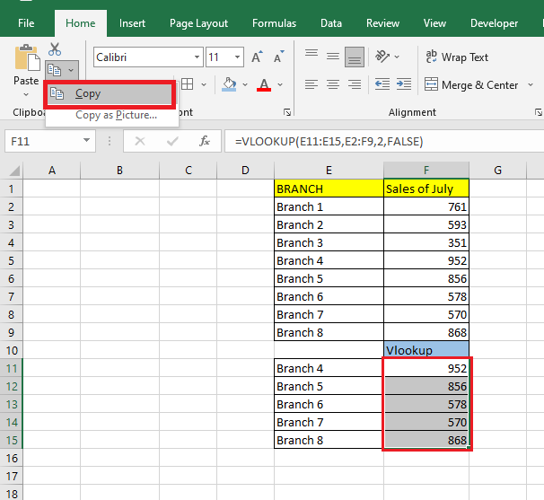
Select all the cells holding VLOOKUP formulas, go to the Home tab, and click Copy in the Clipboard group.
-
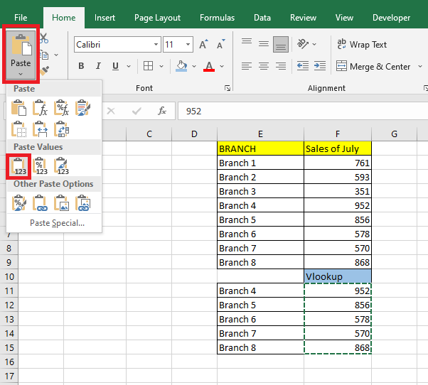
Open the Paste drop-down on the Home tab and choose the Paste Values option, the clipboard icon with 123 on it.
-
Click any of the converted cells. The formula bar now shows a plain value instead of a VLOOKUP formula, and the visible result has not changed.
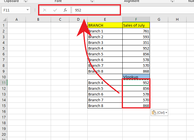
Rule: Paste the values straight back over the cells you copied. Pasting into a different column leaves the original formulas alive and gives you two copies of the same data.
Read also: How to Add Leading Zeros in Microsoft Excel
Method 2: Remove VLOOKUP formulas in multiple sheets
If several worksheets share the same layout, group them first and do the work once.
-
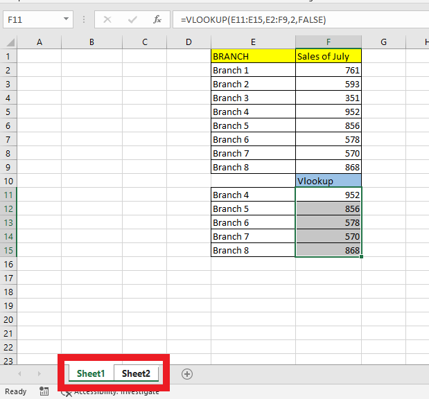
Click the first sheet tab, hold the Shift key, and click the last sheet tab you want to include. The tabs are now grouped.
-
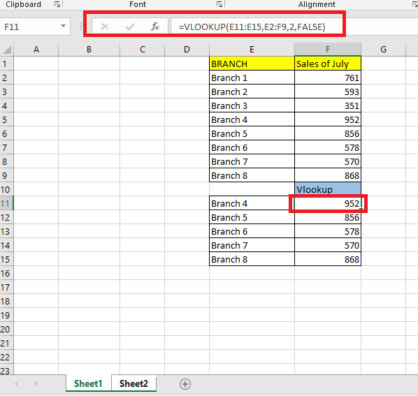
Go to the cells holding the VLOOKUP formulas, for example E11 downwards, and press CTRL+C to copy them.
-
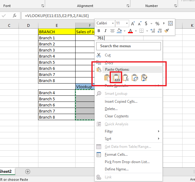
Right-click the same selection, open Paste Options and click Values.
-
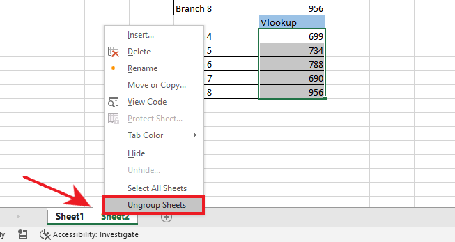
Right-click any sheet tab and choose Ungroup Sheets. Do not skip this. While sheets stay grouped, everything you type lands on all of them.
-
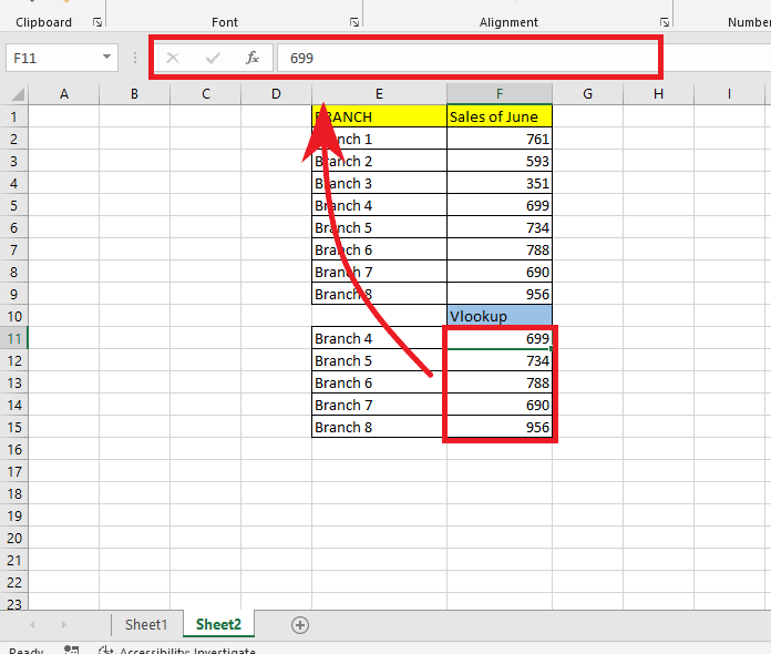
Click into the second sheet and check a cell in the VLOOKUP column. The formula is gone and only the value remains.
Rule: Grouped-sheet edits cannot be undone one sheet at a time. Save a copy of the workbook before you group, and check every sheet afterwards rather than assuming.
Method 3: Go To Special, when you cannot see where the formulas are
On an inherited workbook you often do not know which cells are live and which are typed. Go To Special finds them all for you.
-
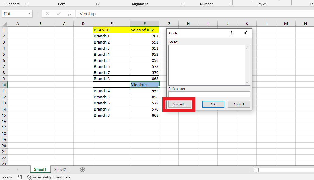
Press CTRL+G to open the Go To dialog box, then click Special. F5 opens the same dialog if you prefer.
-
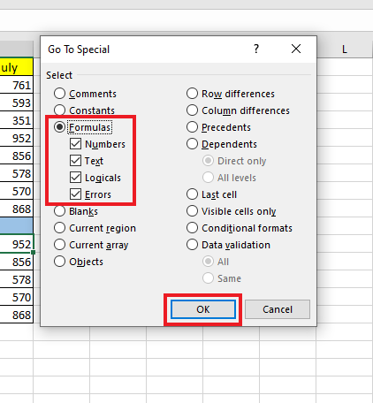
Choose Formulas and click OK. Excel selects every formula cell on the sheet in one go.
-
With that selection still live, press CTRL+C, then open Paste Special, click Values and click OK.
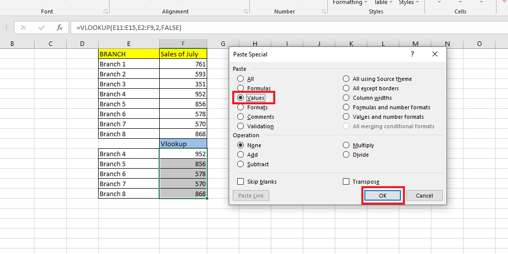
Check the formula bar on any of the cells afterwards. There is no longer a VLOOKUP formula behind it, only the value.
Rule: Go To Special selects every formula on the sheet, not only the VLOOKUP ones. If the sheet also holds SUM totals or IF logic you want to keep, select the lookup column first and Go To Special will confine itself to that selection.
Method 4: The VLOOKUP formula remove shortcut
If you do this often, learn the chain rather than the menu. Select the cells, then:
-
CTRL+C to copy.
-
CTRL+ALT+V to open Paste Special.
-
V to pick Values.
-
Enter to confirm.
Four keystrokes, no mouse, no menu. The older sequence ALT+E+S, then V, then Enter does exactly the same thing and still works in every current Windows build. On a Mac the Paste Special shortcut is CTRL+CMD+V.
Recent Microsoft 365 builds also accept CTRL+SHIFT+V to paste values in one step. If nothing happens when you try it, your build does not have it yet, so use the CTRL+ALT+V route above.
Method 5: Right-drag, no clipboard needed
Select the cells, then hold down the right mouse button on the edge of the selection, drag it where you want it, and release. Excel shows a menu. Choose Copy Here as Values Only. The formulas never make it to the destination. This is the quickest way to remove a formula after VLOOKUP when you also wanted to move the column anyway.
How do you remove a VLOOKUP formula but keep the data?
That is what every method above already does. Paste Values is a swap, not a delete. It takes what the cell was displaying and writes it in as a literal entry, then discards the formula. Nothing you can see on screen changes.
What people usually mean when they ask how to remove a VLOOKUP formula in Excel without losing data is that they tried pressing Delete or Backspace and lost everything. That is the difference:
| What you do | What happens to the formula | What happens to the value |
|---|---|---|
| Press Delete | Removed | Removed too. The cell is empty |
| Clear Contents | Removed | Removed too |
| Paste Values over the selection | Removed | Kept, frozen as a literal entry |
| Delete the source table | Kept, but now broken | Turns into #N/A or #REF! |
So to save VLOOKUP values in Excel permanently, always paste values before you touch the source table. Do it in the wrong order and there is nothing left to save.
Rule: Flatten first, delete second. Once a VLOOKUP has turned into #N/A the original answer is gone and no paste will bring it back.
How do you break a VLOOKUP link to another workbook?
If your VLOOKUP points at a table in a different file, the formula bar shows a file path in square brackets. Removing the formula with Paste Values also removes that dependency, and for a single column that is the simplest answer.
To cut every external link in the workbook at once, go to the Data tab and click Edit Links, called Workbook Links in newer Microsoft 365 builds. Select the source file and choose Break Link. Excel converts every formula that referenced that file into its current value.
Rule: Breaking a link cannot be undone with CTRL+Z. Save a copy of the workbook before you break anything.
How do you hide a VLOOKUP formula instead of removing it?
Sometimes you want the lookup to keep working but you do not want the recipient reading it. Hide it rather than remove it.
-
Select the cells that contain the VLOOKUP formulas.
-
Press CTRL+1 to open Format Cells, go to the Protection tab, and tick Hidden. Leave Locked ticked as well.
-
Go to the Review tab and click Protect Sheet. Set a password if you want one, and click OK.
The cells still calculate, but clicking one shows an empty formula bar. The Hidden tick box on its own does nothing at all until the sheet is protected, which is the step most people miss.
Removing VLOOKUP formulas with a VBA macro
For a workbook with dozens of sheets, or a job you repeat every week, a macro is worth the setup. Press ALT+F11 to open the editor, then Insert and Module, and paste one of these.
To flatten every formula in every sheet:
Sub RemoveAllFormulas()
Dim ws As Worksheet
For Each ws In ThisWorkbook.Worksheets
ws.UsedRange.Value = ws.UsedRange.Value
Next ws
End Sub
To flatten only the cells whose formula actually contains VLOOKUP, on the sheet you are looking at, leaving your SUM and IF formulas alone:
Sub RemoveVlookupOnly()
Dim c As Range
For Each c In ActiveSheet.UsedRange
If c.HasFormula Then
If InStr(1, UCase(c.Formula), "VLOOKUP") > 0 Then c.Value = c.Value
End If
Next c
End Sub
Run it with F5 from the editor, or assign it a shortcut key from the Macros dialog. Microsoft's own getting started with VBA in Office guide covers the editor basics if this is your first macro.
Rule: A macro cannot be undone with CTRL+Z. Test it on a copy of the workbook before you run it on the real one.
Troubleshooting
| What you see | Why | Fix |
|---|---|---|
| The cells went blank after you deleted the formula | You pressed Delete instead of pasting values | Press CTRL+Z immediately, then use Method 1 |
| Paste Special is greyed out | The clipboard is empty, or the marching ants were cancelled | Copy again with CTRL+C and paste before pressing Escape |
| Every cell now shows #N/A | The lookup table moved or was deleted while the formulas were still live | Undo, restore the source data, flatten the lookups, then remove the source |
| Every cell now shows #REF! | A column or sheet the formula pointed at was deleted | Undo. Once #REF! is saved, the original reference cannot be recovered |
| The formulas came back on the other sheets | The sheets were not grouped when you pasted | Regroup with Shift and repeat, or run the macro version |
| The sheet still shows =VLOOKUP(...) as text in every cell | Show Formulas is toggled on | Press CTRL and the grave accent key above Tab to toggle it back |
| Excel typed the VLOOKUP into the whole column again by itself | The range is an Excel Table with a calculated column | Click the small AutoCorrect button that appears and choose Stop Automatically Creating Calculated Columns |
| Values are there but no longer update | Working as intended. That is what removing the formula does | If you need it live again, rewrite the VLOOKUP |
Doing this in Google Sheets instead
The idea is identical but the menu is not. If you searched for how to remove a VLOOKUP formula in Google Sheets, copy the cells, then use Edit and Paste special and Values only, or press CTRL+SHIFT+V. Our full walkthrough is in how to remove a formula and keep the value in Google Sheets.
Final thoughts on removing a VLOOKUP formula in Excel
Removing a VLOOKUP formula is a two-part idea: copy, then paste back as values. Everything else on this page is a variation for a different situation, whether that is several sheets at once, formulas you cannot find, or a job you would rather hand to a macro.
If you want to strip out other kinds of formulas as well, our guide to how to remove formulas in Excel covers the same ground for the whole workbook rather than one lookup column.
You can visit our home page for more easy-to-follow, step-by-step guides. Check the links in the related articles section for further details about Excel and Google Sheets templates.
Frequently asked questions on removing a VLOOKUP formula in Excel
How do I remove a VLOOKUP formula in Excel and keep the values?
Select the cells, press CTRL+C, then paste them back over the same selection using Paste Special and Values. The displayed results stay exactly as they are and the formula behind them is discarded. Pressing Delete instead would remove the results as well.
What is the shortcut to remove a VLOOKUP formula in Excel?
CTRL+C, then CTRL+ALT+V, then V, then Enter. The older ALT+E+S sequence followed by V and Enter does the same thing. Recent Microsoft 365 builds also support CTRL+SHIFT+V as a one-step paste values.
How do I remove VLOOKUP formulas from several worksheets at once?
Click the first sheet tab, hold Shift and click the last one to group them, then copy the lookup cells and paste them back as values. Right-click a tab and choose Ungroup Sheets when you are finished, and check each sheet before you save.
Why is my spreadsheet showing the VLOOKUP formula instead of the result?
Usually Show Formulas is switched on, so press CTRL and the grave accent key above Tab to toggle it off. If only one cell is affected, that cell is probably formatted as Text or the entry starts with an apostrophe. Set the format to General and re-enter the cell with F2 and Enter.
How can I stop Excel autofilling my VLOOKUP down the column?
If the range is an Excel Table, Excel creates a calculated column automatically. Click the small AutoCorrect button that appears beside the cell and choose Stop Automatically Creating Calculated Columns. To turn off the function-name dropdown, go to File, Options, Formulas and untick Formula AutoComplete. To disable dragging altogether, go to File, Options, Advanced and untick Enable fill handle and cell drag-and-drop.
Can I use a VBA macro to remove VLOOKUP formulas in Excel?
Yes, and it is the right tool once you are dealing with many sheets. A loop that sets each sheet's UsedRange value equal to itself flattens every formula in the workbook, and a version that tests each cell with HasFormula and InStr for the word VLOOKUP flattens only the lookups. Neither can be undone, so test on a copy.
How do I hide a VLOOKUP formula in Excel without deleting it?
Select the cells, press CTRL+1, tick Hidden on the Protection tab, then protect the sheet from the Review tab. The lookup keeps calculating but the formula bar stays empty. Ticking Hidden alone does nothing until the sheet is protected.
How do I break a VLOOKUP link to another workbook?
For one column, paste values over it. To cut every external reference at once, go to the Data tab, open Edit Links, called Workbook Links in newer builds, select the source file and click Break Link. Breaking links cannot be undone, so save a copy first.

Related Articles:
Want to Make Excel Work for You? Try out 5 Amazing Excel Templates & 5 Unique Lessons
We hate SPAM. We will never sell your information, for any reason.