The SUMIFS Google Sheets Function: Everything You Need To Know

functions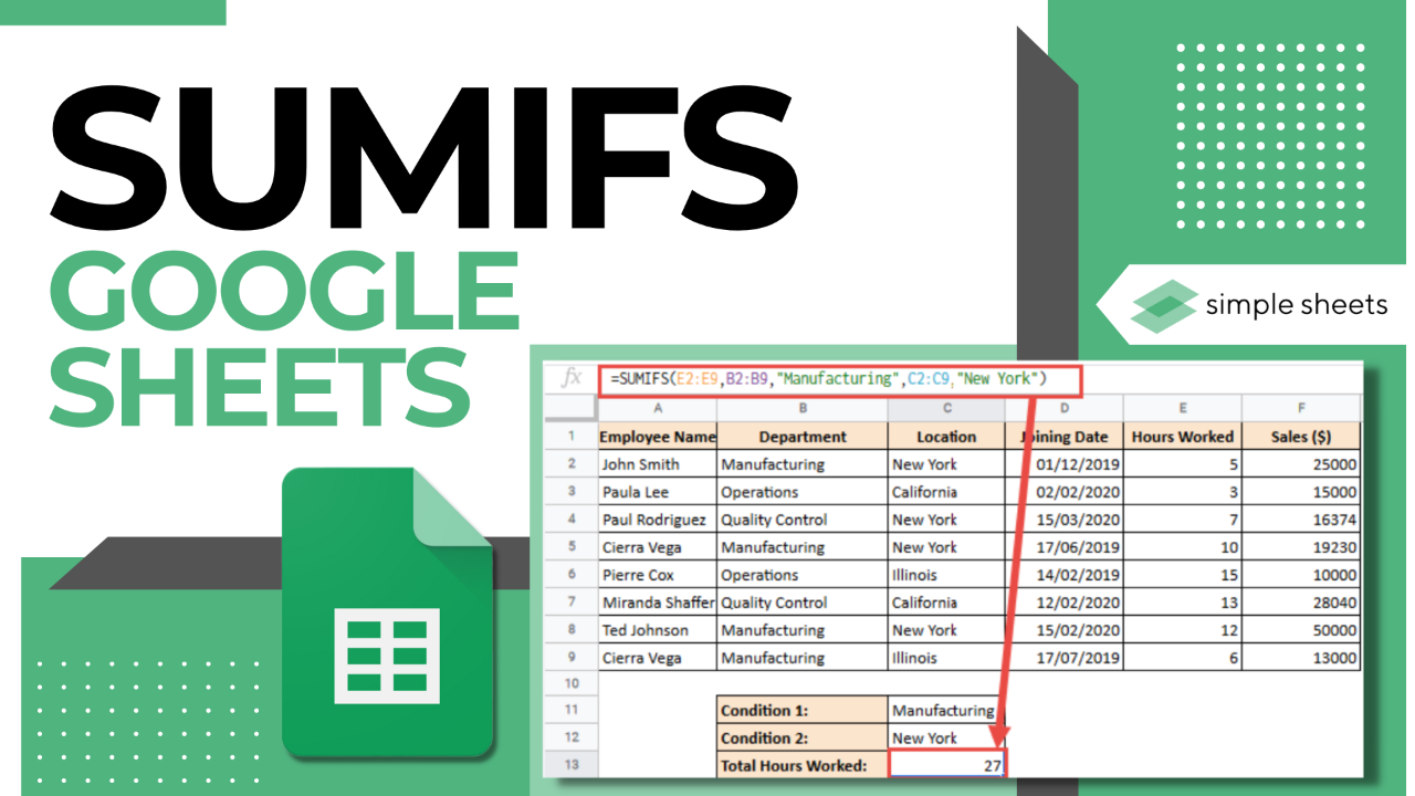 google sheets Feb 22, 2023

Do you want to sum values in your Google Sheets based on preconceived conditions?

The SUMIFS Google Sheets function has got you covered. This function allows you to add numbers depending on multiple criteria.

In this article, we will uncover the following:

The difference between the SUMIF and SUMIFS functions in Google Sheets.
SUM values with multiple criteria.
Other uses of the SUMIFS Google Sheets Function.
Sum Values With Multiple Criteria in Separate Columns
Final Thoughts on the SUMIFS Google Sheets Function
Frequently Asked Questions on the SUMIFS Google Sheets Function
Related Articles

The Difference Between SUMIF and SUMIFS Functions in Google Sheets.

SUMIF can help you add up cells that only meet one condition.
SUMIFS can help you add up cells that meet two or more conditions.
SUMIF Formula =SUMIF(criterion_range,"criterion",sum_range)
SUMIFS Formula =SUMIFS(sum_range,criteria_range1,"criterion1",criteria_range2,"criterion2",...)

SUM Values With Multiple Criteria.

Let's define our arguments:

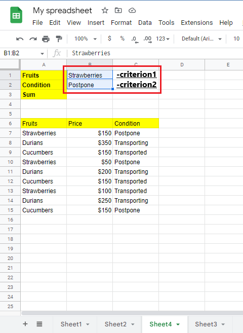
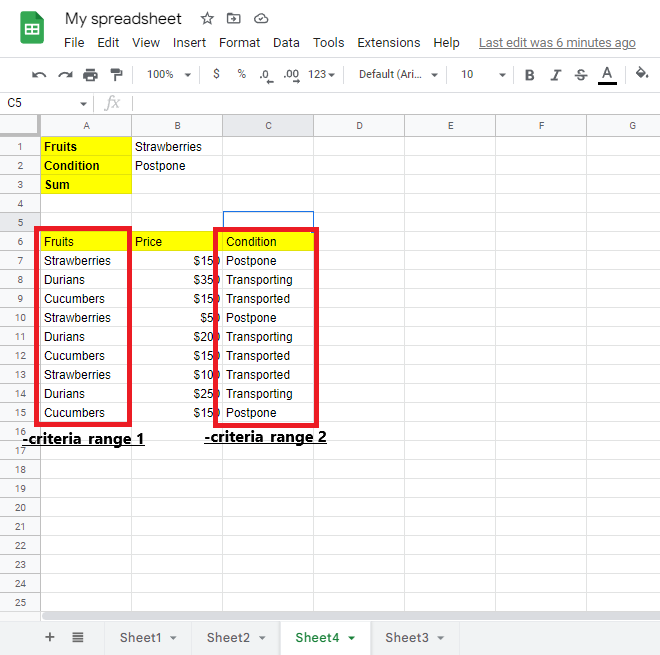
In Column A, typing in "Strawberries" is the first criterion. Now we will use rows 7 to 15 as our criteria_range1. The cells in this range are A7:A17. Our criterion 1 is "Strawberries."
The word "Postpone" should be in column C. It means our criteria_range2 is from C7 to C15, and criterion2 is "Postpone."
The numbers we want to add up are in column B. So our sum_range is from B7 to B15.

When we put all the arguments together, we get a simple formula:

=SUMIFS(B7:B15, A7:A17, "strawberries", C7:C15,"postpone")

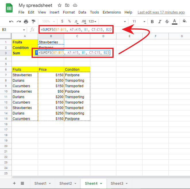
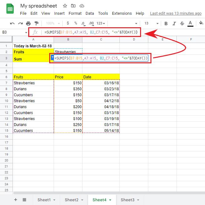
For more flexibility, you can enter both pieces of information in different cells. For example, you could enter the information in cells B1 and B2. Then you can refer to those cells when you need that information.

=SUMIFS(B7:B15, A7:A15, B1, C7:C15, B2)

The steps below show the SUMIFS formula in action.

Prepare your sample data.

Select your criterion1 and criterion2.

Select your Criteria ranges.

Put the SUMIFS formula of the selected criteria column ranges and criteria in cell b3.

Other uses of the SUMIFS Google Sheets Function.

Sometimes, your conditions depend on what other functions say. In this case, put those functions inside the SUMIFS formula.

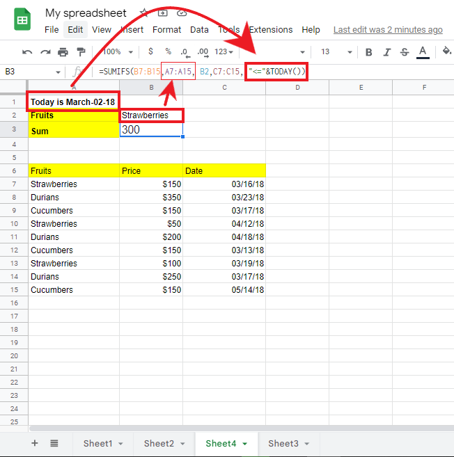
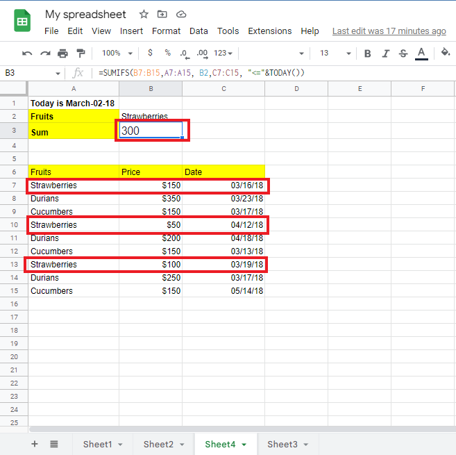
For example, let's sum "strawberries" that are "transported." This means that the transport date is today or earlier. We concatenate the "<=" operator with the TODAY() function:

=SUMIFS(B7:B15,A7:A15, B2,C7:C15, "<="&TODAY())

Input your selected date and the fruit you want to get its sum.

After completing the SUMIFS formula, press enter.

These are the sum of the strawberries transported using the following formula.

SUMIFS With Blank Cells and Non-Blank Cells.

Use one of the following criteria depending on whether another column is a blank cell or a non-blank cell:

"=" is used to sum blank cells. This means that there is nothing in the cell.
"<>" To sum non-blank cells, including zero-length strings.
"To sum up, blank cells include zero-length strings.

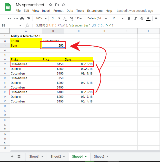
If some dates are missing in the Transported Date column, you can still sum the "strawberries" by only adding the ones with a date listed. You can do this by using this formula:

=SUMIFS(B7:B15,A7:A15,"strawberries" ,C7:C15, "<>")

Sum Values With Multiple Criteria in Separate Columns.

The example below shows how to add numbers when the following logic determines several conditions.

All the conditions in each set must be proper. (AND logic)
A cell is added up if any set of conditions is actual. (OR logic)

To illustrate better, here is an example.

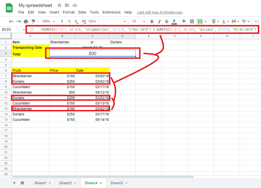
In our sales data set, let's say you want to add up the numbers in column B if column A has either "Strawberries" OR "Durians," AND the date in column C is "2-Mar-2018".

The most obvious way to accomplish this is to make two SUMIFS formulas. One formula will sum "strawberries," and the other will sum "durians."

Then, you can add up the results of both formulas to get the total amount of the selected multiple columns.

=SUMIFS(B7:B15, A7:A15, "strawberries", C7:C15, "2-Mar-2018") + SUMIFS(B7:B15, A7:A15, "durians", C7:C15, "2-Mar-2018")

Final Thoughts on the SUMIFS Google Sheets Function.

Now you have the skills to use the SUMIFS function to make your spreadsheet way more organized.

You can visit our home page for more easy-to-follow how-to and step-by-step guides. Check the links in related articles for further details about Excel/Google Sheets Templates!

Frequently Asked Questions on the SUMIFS Google Sheets Function:

What is causing SUMIFS to malfunction?

The SUMIF function may not work because the data isn't formatted evenly.

Is the SUMIFS function the best way to check all the information in a range?

LOOKUP and INDEX-MATCH (type 1) are the fastest ways to find information.

What function is comparable to the SUMIFS feature in Google Sheets?

The SUMPRODUCT option is similar to the SUMIFS formula because you can add values based on multiple conditions. It works well when there is only one possible match.

Google Sheets Countif: Everything You Need To Know

How to Sum a Column in Google Sheets:4 Easy Methods

Excel Countif Function: Simple Guide For Beginners

Want to Make Excel Work for You? Try out 5 Amazing Excel Templates & 5 Unique Lessons

We hate SPAM. We will never sell your information, for any reason.